Problems tagged with "quiz-04"
Problem #058
Tags: pca, projection, quiz-04, dimensionality reduction, lecture-06
Suppose the direction of maximum variance in a centered data set is
Let \(\vec x = (2, 4)^T\) be a centered data point.
Reduce \(\vec x\) to one dimension by projecting onto the direction of maximum variance. What is the new feature \(z\) obtained from this projection?
Solution
\(z = 3\sqrt 2\).
The projection onto the direction of maximum variance is given by the dot product with \(\vec u\):
Problem #059
Tags: pca, projection, quiz-04, dimensionality reduction, lecture-06
Suppose the direction of maximum variance in a centered data set is
Let \(\vec x = (2, 1, 2)^T\) be a centered data point.
Reduce \(\vec x\) to one dimension by projecting onto the direction of maximum variance. What is the new feature \(z\) obtained from this projection?
Solution
\(z = 3\).
The projection onto the direction of maximum variance is given by the dot product with \(\vec u\):
Problem #060
Tags: pca, projection, quiz-04, dimensionality reduction, lecture-06
Suppose the direction of maximum variance in a centered data set is
Let \(\vec x = (3, 1, -1, 5)^T\) be a centered data point.
Reduce \(\vec x\) to one dimension by projecting onto the direction of maximum variance. What is the new feature \(z\) obtained from this projection?
Solution
\(z = 4\).
The projection onto the direction of maximum variance is given by the dot product with \(\vec u\):
Problem #061
Tags: pca, centering, covariance, quiz-04, lecture-06
Center the data set:
Solution
First, compute the mean:
Then subtract the mean from each data point:
Problem #062
Tags: pca, centering, covariance, quiz-04, lecture-06
Center the data set:
Solution
First, compute the mean:
Then subtract the mean from each data point:
Problem #063
Tags: quiz-04, covariance, lecture-06
Consider the dataset of four points in \(\mathbb R^2\) shown below:
Calculate the sample covariance matrix.
Solution
First, compute the mean:
Then form the centered data matrix \(Z\), whose rows are the centered data points:
The sample covariance matrix is:
Problem #064
Tags: quiz-04, covariance, lecture-06
Consider the data set in the image shown below:
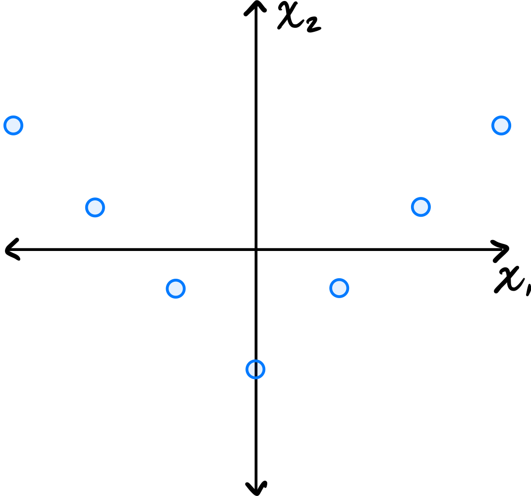
You may assume that this data is already centered and that the symmetry over the \(x_2\) axis is exact.
Which one of the following is true about the \((1, 2)\) entry of the data's sample covariance matrix?
Consider the \((1, 2)\) entry of the covariance matrix, which represents the covariance between the first and second features.
Is the \((1, 2)\) entry of the covariance matrix positive, negative, or zero?
Solution
It is zero.
Because of the symmetry over the \(x_2\) axis, for every point \((a, b)\) in the data set, there is a corresponding point \((-a, b)\). When computing the \((1, 2)\) entry of the covariance matrix, we sum \(\tilde{x}_1^{(i)}\cdot\tilde{x}_2^{(i)}\) over all points. For the symmetric pairs \((a, b)\) and \((-a, b)\), these contributions are \(ab\) and \(-ab\), which cancel out. Therefore, the \((1, 2)\) entry is zero.
Problem #065
Tags: quiz-04, covariance, lecture-06
Let \(\vec{x}^{(1)}, \ldots, \vec{x}^{(6)}\) be a data set of \(6\) points in \(\mathbb R^3\). Shown below are scatter plots of each pair of coordinates (pay close attention to the axis labels):
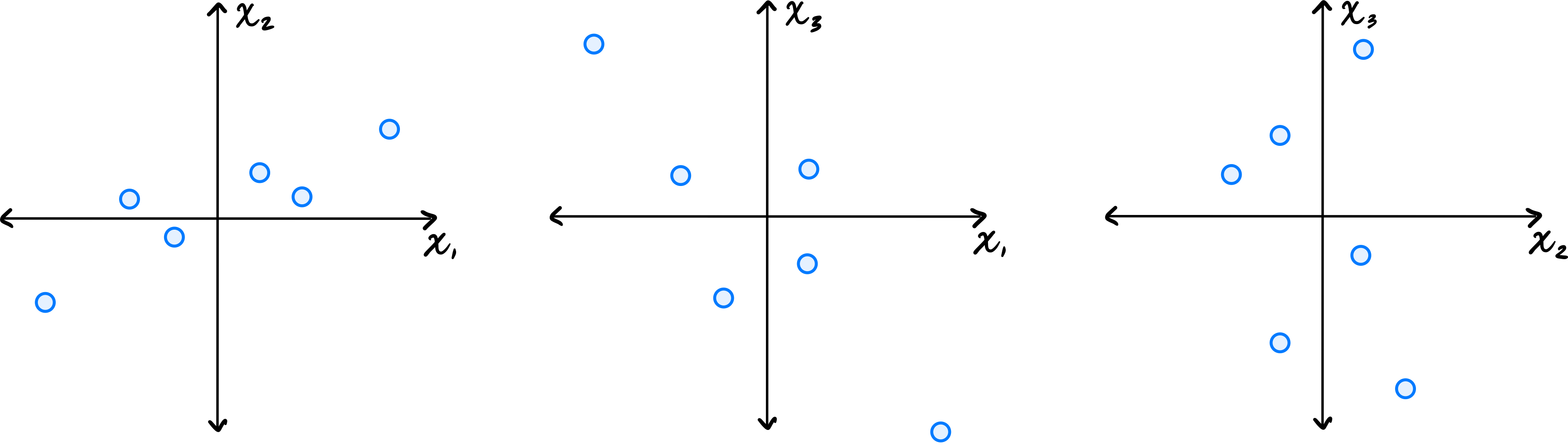
Which one of the following could possibly be the data's sample covariance matrix?
Solution
\(\begin{pmatrix} 10 & 4 & -2 \\ 4 & 5 & 0 \\ -2 & 0 & 10\end{pmatrix}\) From the scatter plots, we can determine the signs of the covariances. The \((x_1, x_2)\) plot shows a positive correlation, so \(C_{12} > 0\). The \((x_1, x_3)\) plot shows a negative correlation, so \(C_{13} < 0\). The \((x_2, x_3)\) plot shows no clear correlation, so \(C_{23}\approx 0\). The only matrix with \(C_{12} > 0\), \(C_{13} < 0\), and \(C_{23} = 0\) is the third choice.
Problem #066
Tags: quiz-04, linear transformations, covariance, lecture-06
Let \(\mathcal X = \{\vec{x}^{(1)}, \ldots, \vec{x}^{(n)}\}\) be a centered data set of \(n\) points in \(\mathbb R^2\). Consider the linear transformation \(\vec f(\vec x) = (-x_1, x_2)^T\), which takes an input point and ``flips'' it over the \(x_2\) axis. Let \(\mathcal X' = \{\vec f(\vec{x}^{(1)}), \ldots, \vec f(\vec{x}^{(n)}) \}\) be the set of points in \(\mathbb R^2\) obtained by applying \(\vec f\) to each point in \(\mathcal X\).
Suppose the sample covariance matrix of \(\mathcal X\) is
What is the sample covariance matrix of \(\mathcal X'\)?
Solution
\(\begin{pmatrix} 5 & 3\\ 3 & 4 \end{pmatrix}\) Flipping the data over the \(x_2\) axis doesn't change the variance (spread) in the \(x_1\) or \(x_2\) directions, and so the diagonal entries of the covariance matrix remain the same. The covariance between \(x_1\) and \(x_2\) stays at the same magnitude but changes sign. That is, the covariance goes from \(-3\) to \(3\).
You can see this more formally, too. The transformation takes a point \((x_1, x_2)^T\) to \((-x_1, x_2)^T\). The covariance between \(x_1\) and \(x_2\) in this transformed data is therefore:
Problem #067
Tags: quiz-04, covariance, variance, lecture-06
Suppose \(C = \begin{pmatrix} 5 & -3\\ -3 & 6 \\ \end{pmatrix}\) is the empirical covariance matrix for a centered data set. What is the variance in the direction given by the unit vector \(\vec{u} = \frac{1}{\sqrt2}(-1, 1)^T\)?
Solution
\(17/2\).
The variance in the direction of a unit vector \(\vec{u}\) is given by \(\vec{u}^T C \vec{u}\).
Problem #068
Tags: covariance, eigenvectors, quiz-04, variance, lecture-06
Let \(C\) be the sample covariance matrix of a centered data set, and suppose \(\vec{u}^{(1)}, \vec{u}^{(2)}, \vec{u}^{(3)}\) are normalized eigenvectors of \(C\) with eigenvalues \(\lambda_1 = 9, \lambda_2 = 3, \lambda_3=0\), respectively.
Suppose \(\vec x = \frac{1}{\sqrt 2}\vec{u}^{(1)} + \frac{1}{\sqrt 6}\vec{u}^{(2)} + \frac{1}{\sqrt 3}\vec{u}^{(3)}\). What is the variance in the direction of \(\vec x\)?
Solution
\(5\) Remember that for any unit vector \(\vec u\), the variance in the direction of \(\vec u\) is given by \(\vec u^T C \vec u\). So, for the vector \(\vec x\), we have
Since \(\vec{u}^{(1)}, \vec{u}^{(2)}, \vec{u}^{(3)}\) are eigenvectors of \(C\), the matrix multiplication simplifies:
Problem #069
Tags: lecture-06, quiz-04, eigenvalues, pca
Let \(C\) be the sample covariance matrix of a centered data set \(\mathcal X\) consisting of five points. Suppose that PCA is performed to reduce the dimensionality of \(\mathcal X\) to one dimension. The results are:
What is the largest eigenvalue of \(C\)?
Solution
\(66/5\) The largest eigenvalue of \(C\) equals the variance of the projected data along the first principal component. This data has mean zero (we can verify: \((4 + 3 - 2 + 1 - 6)/5 = 0\)). So the variance is simply:
Problem #070
Tags: lecture-06, quiz-04, eigenvectors, pca
Consider the data set shown below:
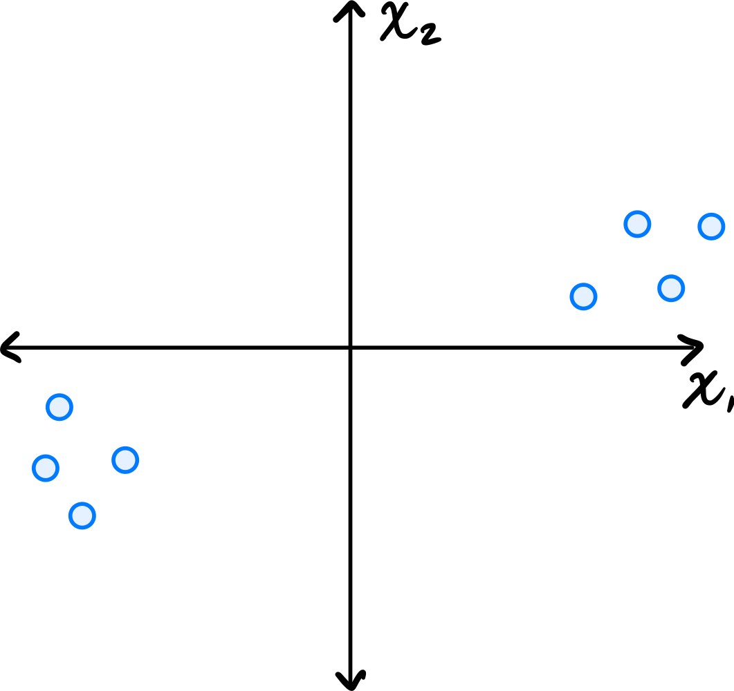
Which of the following could possibly be the top eigenvector of the data's sample covariance matrix?
Solution
\((3, 1)^T\) The top eigenvector of the covariance matrix points in the direction of greatest variance. Looking at the scatter plot, the data is elongated along a direction that has a positive slope, rising more in the \(x_1\) direction than the \(x_2\) direction. The vector \((3, 1)^T\) points roughly in this direction.
\((1, 0)^T\) and \((0, 1)^T\) are along the axes, which don't align with the data's elongation. \((1, 1)^T\) has too steep a slope compared to the apparent direction of the data.
Problem #071
Tags: lecture-07, quiz-04, pca
Let \(\vec{x}^{(1)}\) and \(\vec{x}^{(2)}\) be two points in a centered data set \(\mathcal{X}\) of 100 points in \(d\) dimensions. Suppose PCA is performed, but dimensionality is not reduced; that is, each point \(\vec{x}^{(i)}\) is transformed to the vector \(\vec{z}^{(i)} = U \vec{x}^{(i)}\), where \(U\) is a matrix whose \(d\) rows are the (orthonormal) eigenvectors of the data covariance matrix.
True or False: \(\|\vec{x}^{(1)} - \vec{x}^{(2)}\| = \|\vec{z}^{(1)} - \vec{z}^{(2)}\|\). That is, the distance between \(\vec{z}^{(1)}\) and \(\vec{z}^{(2)}\) in the new data set is necessarily the same as the distance between their corresponding points in the original data set.
Solution
True.
There's a mathematical way of seeing this, and an intuitive way.
Let's start with the intuitive way. We saw in lecture that when we perform PCA without reducing dimensionality, we are simply rotating the data to align with the directions of maximum variance (in the process, "decorrelating" the features). A rotation does not change distances between points, so the distances remain the same. This is illustrated in the figure below. On the left is the original data, and on the right is the same data after PCA transformation (without dimensionality reduction). Notice that the shape of the data hasn't change, and you can find two points in the left plot and see that their distance is the same as the corresponding points in the right plot.
Now for the mathematical way. We want to show that:
We know that \(\vec{z}^{(i)} = U \vec{x}^{(i)}\), so we can rewrite the right-hand side:
Remember that the norm of a vector \(\vec{v}\) can be expressed as:
So:
In the middle of this calculation, we used the fact that \(U\) is an orthonormal matrix, so \(U^T U = I\).
Problem #072
Tags: quiz-04, covariance, variance, lecture-06
Suppose \(C = \begin{pmatrix} 4 & -2\\ -2 & 5 \\ \end{pmatrix}\) is the empirical covariance matrix for a centered data set. What is the variance in the direction given by the unit vector \(\vec{u} = \frac{1}{\sqrt2}(1, 1)^T\)?
Solution
\(5/2\) The variance in the direction of a unit vector \(\vec{u}\) is given by \(\vec{u}^T C \vec{u}\).
Problem #073
Tags: covariance, eigenvectors, quiz-04, variance, lecture-06
Let \(C\) be the sample covariance matrix of a centered data set, and suppose \(\vec{u}^{(1)}, \vec{u}^{(2)}, \vec{u}^{(3)}\) are normalized eigenvectors of \(C\) with eigenvalues \(\lambda_1 = 16, \lambda_2 = 12, \lambda_3=0\), respectively.
Suppose \(\vec x = \frac{1}{\sqrt 2}\vec{u}^{(1)} + \frac{1}{\sqrt 6}\vec{u}^{(2)} + \frac{1}{\sqrt 3}\vec{u}^{(3)}\). What is the variance in the direction of \(\vec x\)?
Solution
\(10\) Remember that for any unit vector \(\vec u\), the variance in the direction of \(\vec u\) is given by \(\vec u^T C \vec u\). So, for the vector \(\vec x\), we have
Since \(\vec{u}^{(1)}, \vec{u}^{(2)}, \vec{u}^{(3)}\) are eigenvectors of \(C\), the matrix multiplication simplifies:
Problem #074
Tags: quiz-04, covariance, lecture-06
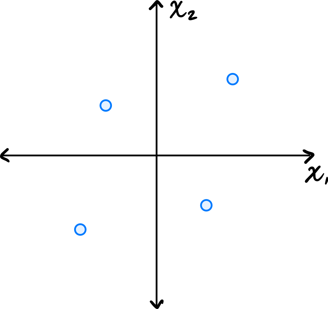
Consider the data set in the image shown below:
You may assume that this data is already centered and that the symmetry over both the \(x_1\) and \(x_2\) axes is exact.
Consider the \((1, 2)\) entry of the data's sample covariance matrix. Is it positive, negative, or zero?
Solution
It is zero.
Because of the symmetry over both the \(x_1\) and \(x_2\) axes, for every point \((a, b)\) in the data set, there are corresponding points \((-a, b)\), \((a, -b)\), and \((-a, -b)\). When computing the \((1, 2)\) entry of the covariance matrix, we sum \(\tilde{x}_1^{(i)}\cdot\tilde{x}_2^{(i)}\) over all points. For these symmetric groups of four points, the contributions are \(ab\), \(-ab\), \(-ab\), and \(ab\), which sum to zero. Therefore, the \((1, 2)\) entry is zero.
Problem #075
Tags: quiz-04, covariance, lecture-06
Consider the dataset of four points in \(\mathbb R^2\) shown below:
Calculate the sample covariance matrix.
Solution
First, compute the mean:
Then form the centered data matrix \(Z\), whose rows are the centered data points:
The sample covariance matrix is:
Problem #076
Tags: quiz-04, linear transformations, covariance, lecture-06
Let \(\mathcal X = \{\vec{x}^{(1)}, \ldots, \vec{x}^{(n)}\}\) be a data set of \(n\) points in \(\mathbb R^2\). Consider the transformation \(\vec f(\vec x) = (x_1 + 5, x_2 - 5)^T\), which takes an input point and ``shifts'' it over by \(5\) units and down by 5 units. Let \(\mathcal X' = \{\vec f(\vec{x}^{(1)}), \ldots, \vec f(\vec{x}^{(n)}) \}\) be the set of points in \(\mathbb R^2\) obtained by applying \(\vec f\) to each point in \(\mathcal X\).
Suppose the sample covariance matrix of \(\mathcal X\) is
What is the sample covariance matrix of \(\mathcal X'\)?
Solution
\(\begin{pmatrix} 5 & -3\\ -3 & 4 \end{pmatrix}\) The transformation \(\vec f(\vec x) = (x_1 + 5, x_2 - 5)^T\) is a translation (shift) of the data. Translations do not affect the covariance matrix, because in defining the covariance matrix we first subtract the mean from each data point. Translating all points shifts the mean by the same amount, so the centered data remains unchanged.
Problem #077
Tags: lecture-06, quiz-04, eigenvalues, pca
Let \(\mathcal X = \{\vec{x}^{(1)}, \ldots, \vec{x}^{(100)}\}\) be a data set of \(100\) points in 50 dimensions. Let \(\lambda\) be the top eigenvalue of the covariance matrix for \(\mathcal X\).
From this data set, we will construct two data sets \(\mathcal A = \{\vec{a}^{(1)}, \ldots, \vec{a}^{(100)}\}\) and \(\mathcal B = \{\vec{b}^{(1)}, \ldots, \vec{b}^{(100)}\}\) in 25 dimensions, by setting \(\vec{a}^{(i)}\) to be the first 25 coordinates of \(\vec{x}^{(i)}\), and setting \(\vec{b}^{(i)}\) to be the remaining 25 coordinates of \(\vec{x}^{(i)}\).
Let \(\lambda_a\) and \(\lambda_b\) be the top eigenvalues of the covariance matrices for \(\mathcal A\) and \(\mathcal B\), respectively.
True or False: it must be the case that \(\lambda = \max\{\lambda_a, \lambda_b\}\).
Solution
False.
The top eigenvalue \(\lambda\) of the full covariance matrix represents the maximum variance in any direction in the 50-dimensional space. This direction may involve correlations between the first 25 and last 25 coordinates.
When we split the data, \(\lambda_a\) captures only the maximum variance within the first 25 dimensions, and \(\lambda_b\) captures only the maximum variance within the last 25 dimensions. Neither can capture variance in directions that span both coordinate sets.
As a counterexample, consider data where all variance is along the direction \((1, 0, \ldots, 0, 1, 0, \ldots, 0)^T\)(a unit vector with components in both the first 25 and last 25 coordinates). The original data would have \(\lambda > 0\), but both \(\mathcal A\) and \(\mathcal B\) would have smaller top eigenvalues, so \(\lambda > \max\{\lambda_a, \lambda_b\}\).
Problem #078
Tags: pca, dimensionality-reduction, eigenvectors, quiz-04, lecture-06
Let \(C\) be the sample covariance matrix of a data set in \(\mathbb{R}^3\), and suppose \(\vec{u}^{(1)}, \vec{u}^{(2)}, \vec{u}^{(3)}\) are orthonormal eigenvectors of \(C\) with eigenvalues \(\lambda_1 = 9, \lambda_2 = 4, \lambda_3 = 1\), respectively, where:
Suppose a data point is \(\vec{x} = \begin{pmatrix} 3 \\ 6 \\ 6 \end{pmatrix}\).
If PCA is performed to reduce the dimensionality from 3 to 2, what is the new representation of \(\vec{x}\)?
Solution
\(\begin{pmatrix} 8 \\ 4 \end{pmatrix}\) In PCA, to reduce from \(d\) dimensions to \(k\) dimensions, we project each data point onto the top \(k\) eigenvectors (those with the largest eigenvalues).
Here, the top 2 eigenvectors are \(\vec{u}^{(1)}\)(with \(\lambda_1 = 9\)) and \(\vec{u}^{(2)}\)(with \(\lambda_2 = 4\)).
The new representation is obtained by computing the dot product of \(\vec{x}\) with each of the top \(k\) eigenvectors:
Therefore, the new representation is:
Problem #079
Tags: pca, dimensionality-reduction, eigenvectors, quiz-04, lecture-06
Let \(C\) be the sample covariance matrix of a data set in \(\mathbb{R}^4\), and suppose \(\vec{u}^{(1)}, \vec{u}^{(2)}, \vec{u}^{(3)}, \vec{u}^{(4)}\) are orthonormal eigenvectors of \(C\) with eigenvalues \(\lambda_1 = 16, \lambda_2 = 9, \lambda_3 = 4, \lambda_4 = 1\), respectively, where:
Suppose a data point is \(\vec{x} = \begin{pmatrix} 3 \\ 3 \\ 6 \\ 6 \end{pmatrix}\).
If PCA is performed to reduce the dimensionality from 4 to 2, what is the new representation of \(\vec{x}\)?
Solution
\(\begin{pmatrix} 9 \\ 1 \end{pmatrix}\) In PCA, to reduce from \(d\) dimensions to \(k\) dimensions, we project each data point onto the top \(k\) eigenvectors (those with the largest eigenvalues).
Here, the top 2 eigenvectors are \(\vec{u}^{(1)}\)(with \(\lambda_1 = 16\)) and \(\vec{u}^{(2)}\)(with \(\lambda_2 = 9\)).
The new representation is obtained by computing the dot product of \(\vec{x}\) with each of the top \(k\) eigenvectors:
Therefore, the new representation is:
Problem #080
Tags: pca, dimensionality-reduction, eigenvectors, quiz-04, lecture-06
Let \(C\) be the sample covariance matrix of a data set in \(\mathbb{R}^5\), and suppose \(\vec{u}^{(1)}, \vec{u}^{(2)}, \vec{u}^{(3)}, \vec{u}^{(4)}, \vec{u}^{(5)}\) are orthonormal eigenvectors of \(C\) with eigenvalues \(\lambda_1 = 25, \lambda_2 = 16, \lambda_3 = 9, \lambda_4 = 4, \lambda_5 = 1\), respectively, where:
Suppose a data point is \(\vec{x} = \begin{pmatrix} 3 \\ 6 \\ 6 \\ 3 \\ 2 \end{pmatrix}\).
If PCA is performed to reduce the dimensionality from 5 to 3, what is the new representation of \(\vec{x}\)?
Solution
\(\begin{pmatrix} 9 \\ 2 \\ 2 \end{pmatrix}\) In PCA, to reduce from \(d\) dimensions to \(k\) dimensions, we project each data point onto the top \(k\) eigenvectors (those with the largest eigenvalues).
Here, the top 3 eigenvectors are \(\vec{u}^{(1)}\)(with \(\lambda_1 = 25\)), \(\vec{u}^{(2)}\)(with \(\lambda_2 = 16\)), and \(\vec{u}^{(3)}\)(with \(\lambda_3 = 9\)).
The new representation is obtained by computing the dot product of \(\vec{x}\) with each of the top \(k\) eigenvectors:
Therefore, the new representation is:
Problem #084
Tags: pca, eigenvectors, quiz-04, dimensionality reduction, lecture-06
Suppose \(C\) is a \(3 \times 3\) sample covariance matrix for a data set \(\mathcal X\), and that the top two eigenvectors of \(C\) are:
with eigenvalues \(\lambda_1 = 10\) and \(\lambda_2 = 4\), respectively.
Let \(\vec x = (1, 2, 3)^T\) be the coordinates of \(\vec x\) with respect to the standard basis. Let \(\vec z\) be the result of applying PCA to reduce the dimensionality of \(\vec x\) to 2. What is \(\vec z\)?
Solution
\(\vec z = \left(\frac{1}{\sqrt 2}, \frac{6}{\sqrt 3}\right)^T\).
We compute \(\vec z\) by projecting \(\vec x\) onto each eigenvector:
Problem #085
Tags: reconstruction error, pca, covariance, eigenvalues, lecture-07, quiz-04
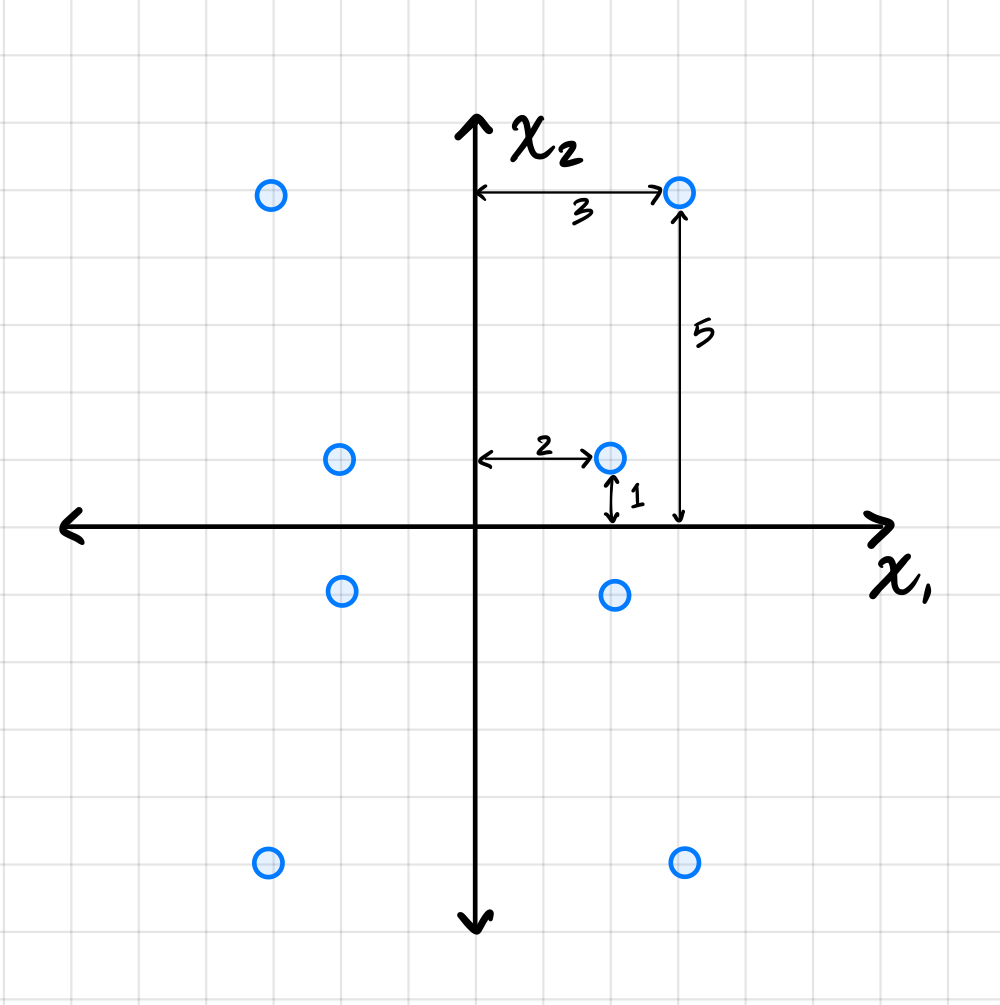
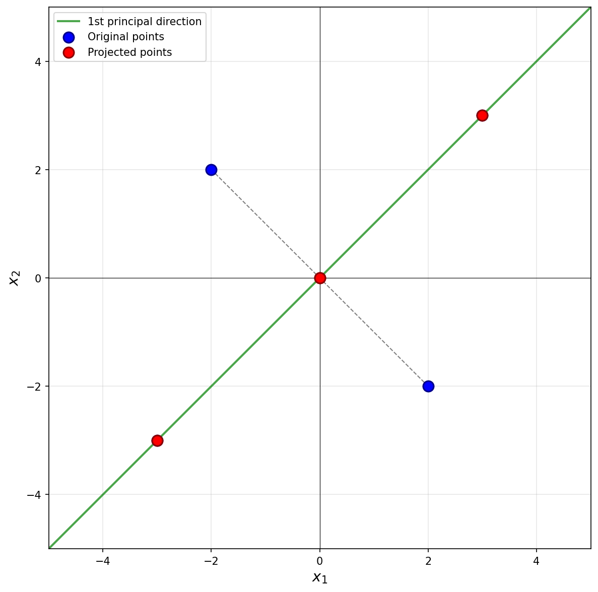
Suppose PCA is used to reduce the dimensionality of the centered data shown below from 2 dimensions to 1.
Part 1)
What will be the reconstruction error?
Solution
\(52\).
The first thing to figure out is what the first principal component (first eigenvector of the covariance matrix) is, since this is the direction onto which the data will be projected. Remember that the first eigenvector points in the direction of maximum variance, and in this plot that appears to be straight up (or down). Thus, the first principal component is \((0, 1)^T\)(or \((0, -1)^T\)).
Next, we imagine projecting all of the data onto this line. Since the first eigenvector is vertical, all of the data is projected onto the \(x_2\)-axis. In the process, every point's \(x_1\)-coordinate is lost, and becomes zero, while the \(x_2\)-coordinate remains unchanged. The figure below shows these projected points in red (note that each red point is actually two points on top of each other, since both \((x_1, x_2)^T\) and \((-x_1, x_2)^T\) project to \((0, x_2)^T\)).
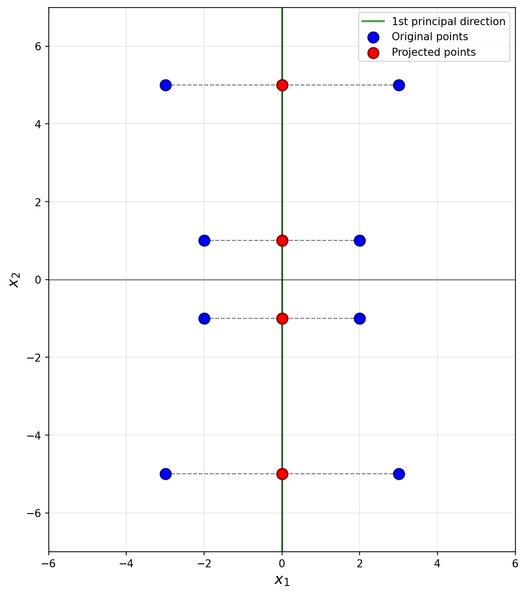
To compute the reconstruction error, we find the squared distance between each point's original position and its projected position. Starting with the upper-right-most point at \((3, 5)^T\), its projection is \((0, 5)^T\), and the squared distance between these two points is \((3 - 0)^2 + (5 - 5)^2 = 9\). For the point at \((2, 1)^T\), its projection is \((0, 1)^T\), and the squared distance is \((2 - 0)^2 + (1 - 1)^2 = 4\).
We could continue, manually calculating the squared distance for each point, but the symmetry of the data allows us to be more efficient. There are four points in the data set that are exactly like the first we just considered and which will have a reconstruction error of 9 each. Similarly, there are four points like the second we considered, each with a reconstruction error of 4. Therefore, the total reconstruction error is:
Part 2)
What is the smallest eigenvalue of the data's covariance matrix?
Solution
\(13/2\).
Remember that the smallest eigenvalue of the data's covariance matrix is equal to the variance of the second PCA feature. That is, it is the variance in the direction of the second principal component (the second eigenvector of the covariance matrix), which in this case is the vector \((1, 0)^T\)(or \((-1, 0)^T\)).
The variance of the data in this direction can be computed by
where \(x_i\) is the \(x_1\)-coordinate of the \(i\)-th data point, \(\mu\) is the mean of all the \(x_1\)-coordinates, and \(n\) is the number of data points. Since hte data is centered, \(\mu = 0\). Therefore, we just need to compute the average of the squared \(x_1\)-coordinates.
Reading these off, we have four points whose \(x_1\)-coordinate is \(3\) or \(-3\), and four points whose \(x_1\)-coordinate is \(2\) or \(-2\). So the variance is:
Therefore, the smallest eigenvalue of the data's covariance matrix is \(13/2\).
Problem #086
Tags: pca, eigenvectors, quiz-04, dimensionality reduction, lecture-06
Suppose \(C\) is a \(3 \times 3\) sample covariance matrix for a data set \(\mathcal X\), and that the top two eigenvectors of \(C\) are:
with eigenvalues \(\lambda_1 = 5\) and \(\lambda_2 = 2\), respectively.
Let \(\vec x = (3,2,1)^T\) be the coordinates of \(\vec x\) with respect to the standard basis. Let \(\vec z\) be the result of applying PCA to reduce the dimensionality of \(\vec x\) to 2. What is \(\vec z\)?
Solution
\(\vec z = \left(0, \frac{3}{\sqrt 2}\right)^T\).
We compute \(\vec z\) by projecting \(\vec x\) onto each eigenvector:
Problem #087
Tags: pca, covariance, eigenvalues, lecture-07, quiz-04
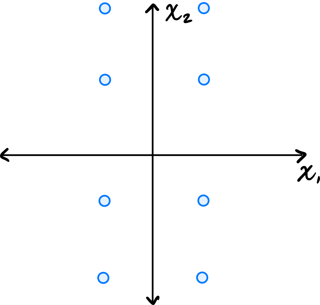
Consider the centered data set shown below. The data is symmetric across both axes.
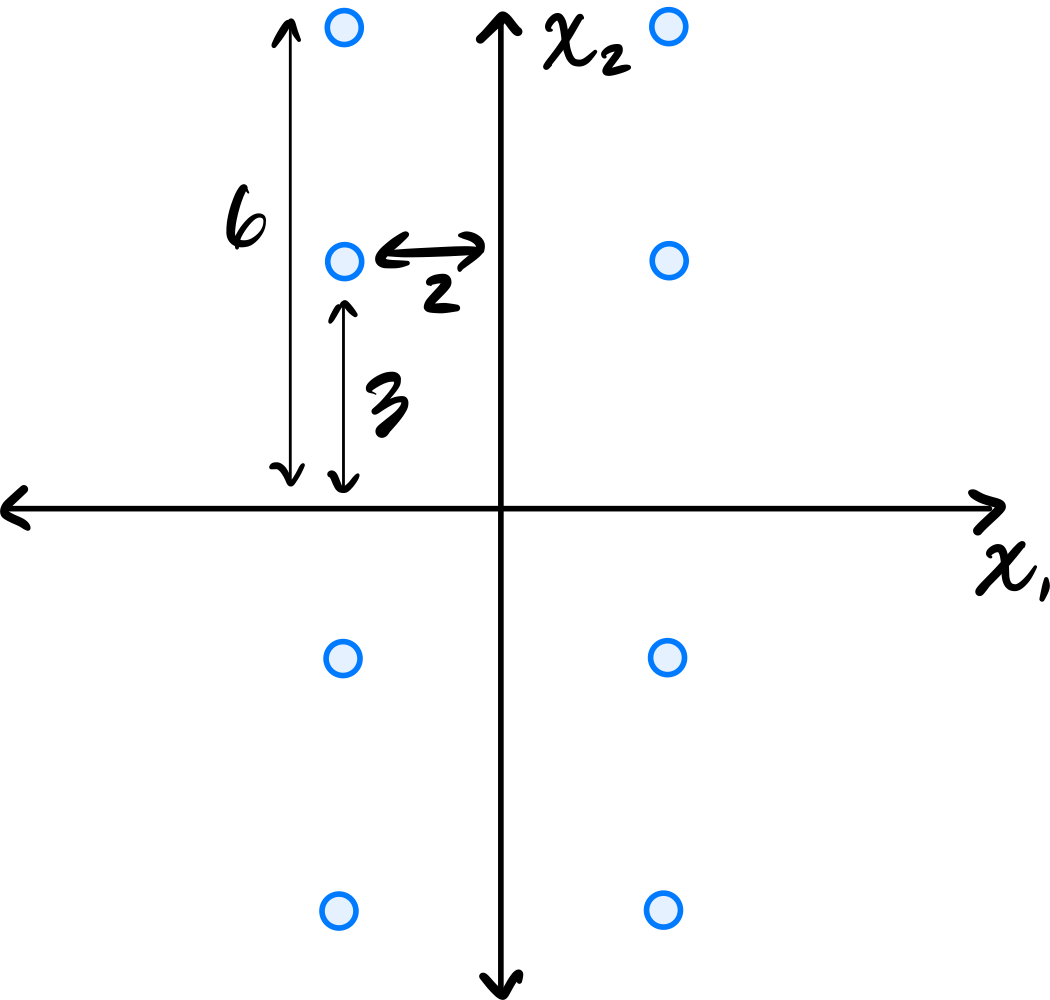
Let \(C\) be the empirical covariance matrix. What is the largest eigenvalue of \(C\)?
Solution
\(45/2\).
Remember that the largest eigenvalue of the data's covariance matrix is equal to the variance of the first PCA feature. That is, it is the variance in the direction of the first principal component (the first eigenvector of the covariance matrix).
Since the data is symmetric across both axes, the eigenvectors of the covariance matrix are aligned with the coordinate axes. From the figure, the data is more spread out vertically than horizontally, so the first principal component is the vector \((0, 1)^T\)(or \((0, -1)^T\)).
The variance of the data in this direction can be computed by
where \(x_i\) is the \(x_2\)-coordinate of the \(i\)-th data point, \(\mu\) is the mean of all the \(x_2\)-coordinates, and \(n\) is the number of data points. Since the data is centered, \(\mu = 0\). Therefore, we just need to compute the average of the squared \(x_2\)-coordinates.
Reading these off, we have four points whose \(x_2\)-coordinate is \(6\) or \(-6\), and four points whose \(x_2\)-coordinate is \(3\) or \(-3\). So the variance is:
Therefore, the largest eigenvalue of the data's covariance matrix is \(45/2\).
Problem #089
Tags: reconstruction error, pca, covariance, eigenvalues, lecture-07, quiz-04
Consider the centered data set consisting of four points:
Suppose PCA is used to reduce the dimensionality of the data from 2 dimensions to 1.
Part 1)
What will be the reconstruction error?
Solution
\(16\).
The first thing to figure out is what the first principal component (first eigenvector of the covariance matrix) is, since this is the direction onto which the data will be projected. Remember that the first eigenvector points in the direction of maximum variance. Looking at the data, the points \((3, 3)^T\) and \((-3, -3)^T\) are farther from the origin than the points \((-2, 2)^T\) and \((2, -2)^T\), so the direction of maximum variance is along the line \(x_2 = x_1\). Thus, the first principal component is \(\frac{1}{\sqrt{2}}(1, 1)^T\)(or \(\frac{1}{\sqrt{2}}(-1, -1)^T\)).
Next, we imagine projecting all of the data onto this line. The figure below shows these projected points in red.
Notice that the points \((3, 3)^T\) and \((-3, -3)^T\) already lie on the line \(x_2 = x_1\), so they project to themselves. Their reconstruction error is zero. The points \((-2, 2)^T\) and \((2, -2)^T\) lie on the line \(x_2 = -x_1\), which is perpendicular to the first principal component. These points both project to the origin \((0, 0)^T\).
To compute the reconstruction error, we find the squared distance between each point's original position and its projected position. For the point at \((-2, 2)^T\), its projection is \((0, 0)^T\), and the squared distance is \((-2 - 0)^2 + (2 - 0)^2 = 4 + 4 = 8\). Similarly, the point \((2, -2)^T\) projects to \((0, 0)^T\) with squared distance \(8\).
Therefore, the total reconstruction error is:
Part 2)
What is the smallest eigenvalue of the data's covariance matrix?
Solution
\(4\).
Remember that the smallest eigenvalue of the data's covariance matrix is equal to the variance of the second PCA feature.
The second PCA feature corresponds to each point's projection onto the second principal component (the second eigenvector of the covariance matrix, and the dashed line in the figure above). In this case, we see that two of the points, \((3, 3)^T\) and \((-3, -3)^T\), project to the origin \((0, 0)^T\), and will have a second PCA feature value of \(0\). The other two points are at \(8\) units away from the origin along this direction, so their second PCA feature values are \(2 \sqrt{2}\) and \(-2 \sqrt{2}\). You could also project these points onto the second principal component to verify this:
Therefore, the second PCA feature values for the four points are 0, 0, 2, and -2. The variance of these (centered) values is:
Problem #090
Tags: lecture-07, quiz-04, dimensionality reduction, pca
Let \(\mathcal X_1\) and \(\mathcal X_2\) be two data sets containing 100 points each, and let \(\mathcal X\) be the combination of the two data sets into a data set of 200 points.
Suppose \(\vec x \in\mathcal X_1\) is a point in the first data set. Suppose PCA is performed on \(\mathcal X_1\) by itself, reducing each point to one dimension, and that the new representation of \(\vec x\) is \(z\).
The point \(\vec x\) is also in the combined data set, \(\mathcal X\). Suppose PCA is performed on the combined data set, \(\mathcal X\), reducing each point to one dimension, and that the new representation of \(\vec x\) after this PCA is \(z'\).
True or False: it is necessarily the case that \(z = z'\).
Solution
False.
The principal eigenvector of \(\mathcal X_1\) may be different from the principal eigenvector of the combined data set \(\mathcal X\). Since \(z\) and \(z'\) are computed by projecting \(\vec x\) onto different eigenvectors, they can be different values.
For example, if \(\mathcal X_1\) has maximum variance along the \(x\)-axis and \(\mathcal X_2\) has maximum variance along the \(y\)-axis, the combined data set might have a different principal direction altogether.
Problem #091
Tags: laplacian eigenmaps, intrinsic dimension, lecture-07, quiz-04, dimensionality reduction
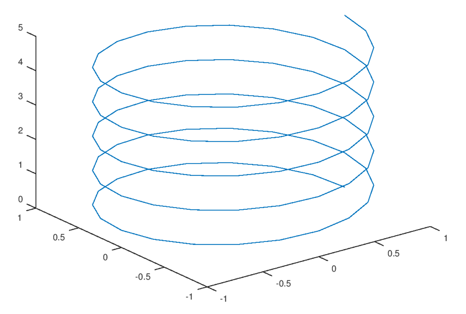
Consider the plot shown below:
Part 1)
What is the ambient dimension?
Solution
3.
The ambient dimension is the dimension of the space in which the data lives. Here, the helix is embedded in 3D space (it has \(x\), \(y\), and \(z\) coordinates), so the ambient dimension is 3.
Part 2)
What is the intrinsic dimension of the curve?
Solution
1.
The intrinsic dimension is the number of parameters needed to describe a point's location on the manifold. For this helix, even though it lives in 3D space, you only need one parameter (e.g., the arc length along the curve, or equivalently, the angle of rotation) to specify any point on it. If you ``unroll'' the helix, it becomes a straight line, which is 1-dimensional. Therefore, the intrinsic dimension is 1.
Problem #092
Tags: laplacian eigenmaps, intrinsic dimension, lecture-07, quiz-04, dimensionality reduction
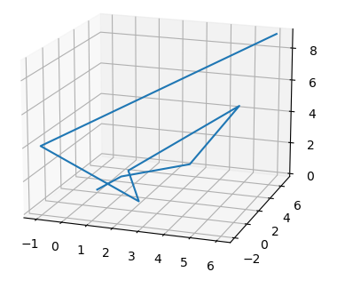
Consider the plot shown below:
Part 1)
What is the ambient dimension?
Solution
3.
The ambient dimension is the dimension of the space in which the data lives. The curve shown is embedded in 3D space (with \(x\), \(y\), and \(z\) axes visible), so the ambient dimension is 3.
Part 2)
What is the intrinsic dimension of the curve?
Solution
1.
The intrinsic dimension is the minimum number of coordinates needed to describe a point's position on the manifold itself. This zigzag path, despite twisting through 3D space, is fundamentally a 1-dimensional curve. You only need a single parameter (such as the distance traveled along the path from a starting point) to uniquely identify any location on it. If you were to ``straighten out'' the path, it would become a line segment, confirming its intrinsic dimension is 1.