Problems tagged with "eigenvalues"
Problem #028
Tags: linear algebra, quiz-03, eigenvalues, eigenvectors, lecture-04
Let \(A = \begin{pmatrix} 3 & 1 \\ 1 & 3 \end{pmatrix}\) and let \(\vec v = (1, 1)^T\).
True or False: \(\vec v\) is an eigenvector of \(A\). If true, what is the corresponding eigenvalue?
Solution
True, with eigenvalue \(\lambda = 4\).
We compute:
Since \(A \vec v = 4 \vec v\), the vector \(\vec v\) is an eigenvector with eigenvalue \(4\).
Problem #029
Tags: linear algebra, quiz-03, eigenvalues, eigenvectors, lecture-04
Let \(A = \begin{pmatrix} 2 & 1 \\ 1 & 2 \end{pmatrix}\) and let \(\vec v = (1, 2)^T\).
True or False: \(\vec v\) is an eigenvector of \(A\). If true, what is the corresponding eigenvalue?
Solution
False.
We compute:
For \(\vec v\) to be an eigenvector, we would need \(A \vec v = \lambda\vec v\) for some scalar \(\lambda\). This would require:
From the first component, we would need \(\lambda = 4\). From the second component, we would need \(\lambda = \frac{5}{2}\). Since these two values are not equal, there is no such \(\lambda\) that satisfies both equations. Therefore, \(\vec v\) is not an eigenvector of \(A\).
Problem #030
Tags: linear algebra, quiz-03, eigenvalues, eigenvectors, lecture-04
Let \(A = \begin{pmatrix} 1 & 1 & 3 \\ 1 & 2 & 1 \\ 3 & 1 & 9 \end{pmatrix}\) and let \(\vec v = (1, 4, -1)^T\).
True or False: \(\vec v\) is an eigenvector of \(A\). If true, what is the corresponding eigenvalue?
Solution
True, with eigenvalue \(\lambda = 2\).
We compute:
Since \(A \vec v = 2 \vec v\), the vector \(\vec v\) is an eigenvector with eigenvalue \(2\).
Problem #031
Tags: linear algebra, quiz-03, eigenvalues, eigenvectors, lecture-04
Let \(A = \begin{pmatrix} 5 & 1 & 1 & 1 \\ 1 & 5 & 1 & 1 \\ 1 & 1 & 5 & 1 \\ 1 & 1 & 1 & 5 \end{pmatrix}\) and let \(\vec v = (1, 2, -2, -1)^T\).
True or False: \(\vec v\) is an eigenvector of \(A\). If true, what is the corresponding eigenvalue?
Solution
True, with eigenvalue \(\lambda = 4\).
We compute:
Since \(A \vec v = 4 \vec v\), the vector \(\vec v\) is an eigenvector with eigenvalue \(4\).
Problem #032
Tags: linear algebra, quiz-03, eigenvalues, eigenvectors, lecture-04
Let \(A = \begin{pmatrix} 1 & 6 \\ 6 & 6 \end{pmatrix}\) and let \(\vec v = (3, -2)^T\).
True or False: \(\vec v\) is an eigenvector of \(A\). If true, what is the corresponding eigenvalue?
Solution
True, with eigenvalue \(\lambda = -3\).
We compute:
Since \(A \vec v = -3 \vec v\), the vector \(\vec v\) is an eigenvector with eigenvalue \(-3\).
Problem #033
Tags: linear algebra, quiz-03, eigenvalues, eigenvectors, lecture-04
Let \(\vec v\) be a unit vector in \(\mathbb R^d\), and let \(I\) be the \(d \times d\) identity matrix. Consider the matrix \(P\) defined as:
True or False: \(\vec v\) is an eigenvector of \(P\).
Solution
True.
To verify this, we compute \(P \vec v\):
Since \(P \vec v = -\vec v = (-1) \vec v\), we see that \(\vec v\) is an eigenvector of \(P\) with eigenvalue \(-1\).
Note: The matrix \(P = I - 2 \vec v \vec v^T\) is called a Householder reflection matrix, which reflects vectors across the hyperplane orthogonal to \(\vec v\).
Problem #034
Tags: linear algebra, quiz-03, eigenvalues, eigenvectors, lecture-04
Let \(A\) be the matrix:
It can be verified that the vector \(\vec{u}^{(1)} = (2, 1)^T\) is an eigenvector of \(A\).
Part 1)
What is the eigenvalue associated with \(\vec{u}^{(1)}\)?
Solution
The eigenvalue is \(\lambda_1 = 6\).
To find the eigenvalue, we compute \(A \vec{u}^{(1)}\):
Therefore, \(\lambda_1 = 6\).
Part 2)
Find another eigenvector \(\vec{u}^{(2)}\) of \(A\). Your eigenvector should have an eigenvalue that is different from \(\vec{u}^{(1)}\)'s eigenvalue. It does not need to be normalized.
Solution
\(\vec{u}^{(2)} = (1, -2)^T\)(or any scalar multiple).
Since \(A\) is symmetric, we know that we can always find two orthogonal eigenvectors. This suggests that we should find a vector orthogonal to \(\vec{u}^{(1)} = (2, 1)^T\) and make sure that it is indeed an eigenvector.
We know from the math review in Week 01 that the vector \((1, -2)^T\) is orthogonal to \((2, 1)^T\)(in general, \((a, b)^T\) is orthogonal to \((-b, a)^T\)).
We can verify:
So the eigenvalue is \(\lambda_2 = 1\), which is indeed different from \(\lambda_1 = 6\).
Problem #035
Tags: linear algebra, quiz-03, eigenvalues, eigenvectors, lecture-04
Let \(D\) be the diagonal matrix:
Part 1)
What is the top eigenvalue of \(D\)? What eigenvector corresponds to this eigenvalue?
Solution
The top eigenvalue is \(7\).
For a diagonal matrix, the eigenvalues are exactly the diagonal entries. The diagonal entries are \(2, -5, 7\), and the largest is \(7\).
An eigenvector corresponding to this eigenvalue is \(\vec v = (0, 0, 1)^T\).
Part 2)
What is the bottom (smallest) eigenvalue of \(D\)? What eigenvector corresponds to this eigenvalue?
Solution
The bottom eigenvalue is \(-5\).
An eigenvector corresponding to this eigenvalue is \(\vec w = (0, 1, 0)^T\).
Problem #036
Tags: linear algebra, quiz-03, eigenvalues, eigenvectors, lecture-04, linear transformations
Consider the linear transformation \(\vec f : \mathbb{R}^2 \to\mathbb{R}^2\) that reflects vectors over the line \(y = -x\).
Find two orthogonal eigenvectors of this transformation and their corresponding eigenvalues.
Solution
The eigenvectors are \((1, -1)^T\) with \(\lambda = 1\), and \((1, 1)^T\) with \(\lambda = -1\).
Geometrically, vectors along the line \(y = -x\)(i.e., multiples of \((1, -1)^T\)) are unchanged by reflection over that line, so they have eigenvalue \(1\). Vectors perpendicular to the line \(y = -x\)(i.e., multiples of \((1, 1)^T\)) are flipped to point in the opposite direction, so they have eigenvalue \(-1\).
Problem #037
Tags: linear algebra, quiz-03, eigenvalues, eigenvectors, lecture-04, linear transformations
Consider the linear transformation \(\vec f : \mathbb{R}^2 \to\mathbb{R}^2\) that scales vectors along the line \(y = x\) by a factor of 2, and scales vectors along the line \(y = -x\) by a factor of 3.
Find two orthogonal eigenvectors of this transformation and their corresponding eigenvalues.
Solution
The eigenvectors are \((1, 1)^T\) with \(\lambda = 2\), and \((1, -1)^T\) with \(\lambda = 3\).
Geometrically, vectors along the line \(y = x\)(i.e., multiples of \((1, 1)^T\)) are scaled by a factor of 2, so they have eigenvalue \(2\). Vectors along the line \(y = -x\)(i.e., multiples of \((1, -1)^T\)) are scaled by a factor of 3, so they have eigenvalue \(3\).
Problem #038
Tags: linear algebra, quiz-03, eigenvalues, eigenvectors, lecture-04, linear transformations
Consider the linear transformation \(\vec f : \mathbb{R}^2 \to\mathbb{R}^2\) that rotates vectors by \(180°\).
Find two orthogonal eigenvectors of this transformation and their corresponding eigenvalues.
Solution
Any pair of orthogonal vectors works, such as \((1, 0)^T\) and \((0, 1)^T\). Both have eigenvalue \(\lambda = -1\).
Geometrically, rotating any vector by \(180°\) reverses its direction, so \(\vec f(\vec v) = -\vec v\) for all \(\vec v\). This means every nonzero vector is an eigenvector with eigenvalue \(-1\).
Since we need two orthogonal eigenvectors, any orthogonal pair will do.
Problem #039
Tags: linear algebra, quiz-03, eigenvalues, eigenvectors, lecture-04
Consider the diagonal matrix:
How many unit length eigenvectors does \(A\) have?
Solution
\(\infty\) The upper-left \(2 \times 2\) block of \(A\) is the identity matrix. Recall from lecture that the identity matrix has infinitely many eigenvectors: every nonzero vector is an eigenvector of the identity with eigenvalue 1.
Similarly, any vector of the form \((a, b, 0)^T\) where \(a\) and \(b\) are not both zero satisfies:
So any such vector is an eigenvector with eigenvalue 1. There are infinitely many unit vectors of this form (they form a circle in the \(x\)-\(y\) plane), so \(A\) has infinitely many unit length eigenvectors.
Additionally, \((0, 0, 1)^T\) is an eigenvector with eigenvalue 5.
Problem #045
Tags: linear algebra, eigenbasis, quiz-03, eigenvalues, eigenvectors, lecture-04
Let \(\vec{u}^{(1)}, \vec{u}^{(2)}, \vec{u}^{(3)}\) be three unit length orthonormal eigenvectors of a linear transformation \(\vec{f}\), with eigenvalues \(8\), \(4\), and \(-3\) respectively.
Suppose a vector \(\vec{x}\) can be written as:
What is \(\vec{f}(\vec{x})\), expressed in coordinates with respect to the eigenbasis \(\{\vec{u}^{(1)}, \vec{u}^{(2)}, \vec{u}^{(3)}\}\)?
Solution
\([\vec{f}(\vec{x})]_{\mathcal{U}} = (16, -12, -3)^T\) Using linearity and the eigenvector property:
Since \(\vec{u}^{(1)}\) is an eigenvector with eigenvalue \(8\), we have \(\vec{f}(\vec{u}^{(1)}) = 8\vec{u}^{(1)}\). Similarly, \(\vec{f}(\vec{u}^{(2)}) = 4\vec{u}^{(2)}\) and \(\vec{f}(\vec{u}^{(3)}) = -3\vec{u}^{(3)}\):
In the eigenbasis, this is simply \((16, -12, -3)^T\).
Problem #046
Tags: linear algebra, eigenbasis, quiz-03, eigenvalues, eigenvectors, lecture-04
Let \(\vec{u}^{(1)}, \vec{u}^{(2)}, \vec{u}^{(3)}\) be three unit length orthonormal eigenvectors of a linear transformation \(\vec{f}\), with eigenvalues \(5\), \(-2\), and \(3\) respectively.
Suppose a vector \(\vec{x}\) can be written as:
What is \(\vec{f}(\vec{x})\), expressed in coordinates with respect to the eigenbasis \(\{\vec{u}^{(1)}, \vec{u}^{(2)}, \vec{u}^{(3)}\}\)?
Solution
\([\vec{f}(\vec{x})]_{\mathcal{U}} = (20, -2, -6)^T\) Using linearity and the eigenvector property:
Since \(\vec{u}^{(1)}\) is an eigenvector with eigenvalue \(5\), we have \(\vec{f}(\vec{u}^{(1)}) = 5\vec{u}^{(1)}\). Similarly, \(\vec{f}(\vec{u}^{(2)}) = -2\vec{u}^{(2)}\) and \(\vec{f}(\vec{u}^{(3)}) = 3\vec{u}^{(3)}\):
In the eigenbasis, this is simply \((20, -2, -6)^T\).
Problem #047
Tags: optimization, linear algebra, quiz-03, eigenvalues, eigenvectors, lecture-04
Let \(A\) be a symmetric matrix with eigenvalues \(6\) and \(-9\).
True or False: The maximum value of \(\|A\vec{x}\|\) over all unit vectors \(\vec{x}\) is \(6\).
Solution
False. The maximum is \(9\).
The maximum of \(\|A\vec{x}\|\) over unit vectors is achieved when \(\vec{x}\) is an eigenvector corresponding to the eigenvalue with the largest absolute value.
Here, \(|-9| = 9 > 6 = |6|\), so the maximum is achieved at the eigenvector with eigenvalue \(-9\).
If \(\vec{u}\) is a unit eigenvector with eigenvalue \(-9\), then:
Problem #048
Tags: optimization, linear algebra, quiz-03, eigenvalues, eigenvectors, quadratic forms, lecture-04
Let \(A\) be a \(3 \times 3\) symmetric matrix with the following eigenvectors and corresponding eigenvalues: \(\vec{u}^{(1)} = \frac{1}{3}(1, 2, 2)^T\) has eigenvalue \(4\), \(\vec{u}^{(2)} = \frac{1}{3}(2, 1, -2)^T\) has eigenvalue \(1\), and \(\vec{u}^{(3)} = \frac{1}{3}(2, -2, 1)^T\) has eigenvalue \(-10\).
Consider the quadratic form \(\vec{x}\cdot A\vec{x}\).
Part 1)
What unit vector \(\vec{x}\) maximizes \(\vec{x}\cdot A\vec{x}\)?
Solution
\(\vec{u}^{(1)} = \frac{1}{3}(1, 2, 2)^T\) The quadratic form \(\vec{x}\cdot A\vec{x}\) is maximized by the eigenvector with the largest eigenvalue. Among \(4\), \(1\), and \(-10\), the largest is \(4\), so the maximizer is \(\vec{u}^{(1)}\).
Part 2)
What is the maximum value of \(\vec{x}\cdot A\vec{x}\) over all unit vectors?
Solution
\(4\) The maximum value equals the largest eigenvalue. We can verify:
Part 3)
What unit vector \(\vec{x}\) minimizes \(\vec{x}\cdot A\vec{x}\)?
Solution
\(\vec{u}^{(3)} = \frac{1}{3}(2, -2, 1)^T\) The quadratic form is minimized by the eigenvector with the smallest eigenvalue. Among \(4\), \(1\), and \(-10\), the smallest is \(-10\), so the minimizer is \(\vec{u}^{(3)}\).
Part 4)
What is the minimum value of \(\vec{x}\cdot A\vec{x}\) over all unit vectors?
Solution
\(-10\) The minimum value equals the smallest eigenvalue. We can verify:
Problem #049
Tags: linear algebra, quiz-03, eigenvalues, eigenvectors, lecture-04
Let \(A\) be a symmetric matrix with top eigenvalue \(\lambda\). Let \(B = A + 5I\), where \(I\) is the identity matrix.
True or False: The top eigenvalue of \(B\) must be \(\lambda + 5\).
Solution
True.
The main thing to realize is that \(A\) and \(B\) have the same eigenvectors. If \(\vec v\) is an eigenvector of \(A\) with eigenvalue \(\lambda\), then:
Thus, \(\vec v\) is also an eigenvector of \(B\) with eigenvalue \(\lambda + 5\).
This means that the eigenvalues of \(B\) are simply the eigenvalues of \(A\) shifted by 5. Therefore, if \(\lambda\) is the top eigenvalue of \(A\), then \(\lambda + 5\) is the top eigenvalue of \(B\).
Problem #053
Tags: linear algebra, quiz-03, lecture-05, eigenvalues, eigenvectors, diagonalization
Let \(\vec f\) be a linear transformation with eigenvectors and eigenvalues:
What is \(\vec f(\vec x)\) for \(\vec x = (3, 1)^T\)?
Solution
\(\vec f(\vec x) = (3, 5)^T\).
We'll take the three step approach of 1) finding the coordinates of \(\vec x\) in the eigenbasis, 2) applying the transformation in that basis (where the matrix of the transformation \(A_\mathcal{U}\) is diagonal and consists of the eigenvalues), and 3) converting back to the standard basis.
We saw in lecture that we can do this all in one go using the change of basis matrix \(U\):
where \(U\) is the change of basis matrix with the eigenvectors as rows and \(A_\mathcal{U}\) is the diagonal matrix with the eigenvalues on the diagonal. In this case, they are:
Then:
Problem #054
Tags: linear algebra, quiz-03, lecture-05, eigenvalues, eigenvectors, diagonalization
Let \(\vec f\) be a linear transformation with eigenvectors and eigenvalues:
What is \(\vec f(\vec x)\) for \(\vec x = (1, 1, 2)^T\)?
Solution
\(\vec f(\vec x) = (3, 3, 2)^T\).
We'll take the three step approach of 1) finding the coordinates of \(\vec x\) in the eigenbasis, 2) applying the transformation in that basis (where the matrix of the transformation \(A_\mathcal{U}\) is diagonal and consists of the eigenvalues), and 3) converting back to the standard basis.
We saw in lecture that we can do this all in one go using the change of basis matrix \(U\):
where \(U\) is the change of basis matrix with the eigenvectors as rows and \(A_\mathcal{U}\) is the diagonal matrix with the eigenvalues on the diagonal. In this case, they are:
Then:
Problem #055
Tags: linear algebra, quiz-03, lecture-05, eigenvalues, eigenvectors, diagonalization
Let \(\vec f\) be a linear transformation with eigenvectors and eigenvalues:
What is \(\vec f(\vec x)\) for \(\vec x = (4, 0, 0, 0)^T\)?
Solution
\(\vec f(\vec x) = (7, 5, 3, 1)^T\).
We'll take the three step approach of 1) finding the coordinates of \(\vec x\) in the eigenbasis, 2) applying the transformation in that basis (where the matrix of the transformation \(A_\mathcal{U}\) is diagonal and consists of the eigenvalues), and 3) converting back to the standard basis.
We saw in lecture that we can do this all in one go using the change of basis matrix \(U\):
where \(U\) is the change of basis matrix with the eigenvectors as rows and \(A_\mathcal{U}\) is the diagonal matrix with the eigenvalues on the diagonal. In this case, they are:
Then:
Problem #056
Tags: linear algebra, quiz-03, symmetric matrices, spectral theorem, eigenvalues, eigenvectors, lecture-05
Find a symmetric \(2 \times 2\) matrix \(A\) whose eigenvectors are \(\hat{u}^{(1)} = \frac{1}{\sqrt{5}}(1, 2)^T\) with eigenvalue \(6\) and \(\hat{u}^{(2)} = \frac{1}{\sqrt{5}}(2, -1)^T\) with eigenvalue \(1\).
Solution
\(A = \begin{pmatrix} 2 & 2 \\ 2 & 5 \end{pmatrix}\).
We saw in lecture that a symmetric matrix \(A\) can be written as \(A = U^T \Lambda U\), where \(U\) is the matrix whose rows are the eigenvectors of \(A\) and \(\Lambda\) is the diagonal matrix of eigenvalues.
This means that if we know the eigenvectors and eigenvalues of a symmetric matrix, we can "work backwards" to find the matrix itself.
In this case:
Therefore:
Problem #057
Tags: linear algebra, quiz-03, symmetric matrices, spectral theorem, eigenvalues, eigenvectors, lecture-05
Find a symmetric \(3 \times 3\) matrix \(A\) whose eigenvectors are \(\hat{u}^{(1)} = \frac{1}{3}(1, 2, 2)^T\) with eigenvalue \(9\), \(\hat{u}^{(2)} = \frac{1}{3}(2, 1, -2)^T\) with eigenvalue \(18\), and \(\hat{u}^{(3)} = \frac{1}{3}(2, -2, 1)^T\) with eigenvalue \(-9\).
Solution
\(A = \begin{pmatrix} 5 & 10 & -8 \\ 10 & 2 & 2 \\ -8 & 2 & 11 \end{pmatrix}\).
We saw in lecture that a symmetric matrix \(A\) can be written as \(A = U^T \Lambda U\), where \(U\) is the matrix whose rows are the eigenvectors of \(A\) and \(\Lambda\) is the diagonal matrix of eigenvalues.
In this case:
Therefore:
Problem #069
Tags: lecture-06, quiz-04, eigenvalues, pca
Let \(C\) be the sample covariance matrix of a centered data set \(\mathcal X\) consisting of five points. Suppose that PCA is performed to reduce the dimensionality of \(\mathcal X\) to one dimension. The results are:
What is the largest eigenvalue of \(C\)?
Solution
\(66/5\) The largest eigenvalue of \(C\) equals the variance of the projected data along the first principal component. This data has mean zero (we can verify: \((4 + 3 - 2 + 1 - 6)/5 = 0\)). So the variance is simply:
Problem #077
Tags: lecture-06, quiz-04, eigenvalues, pca
Let \(\mathcal X = \{\vec{x}^{(1)}, \ldots, \vec{x}^{(100)}\}\) be a data set of \(100\) points in 50 dimensions. Let \(\lambda\) be the top eigenvalue of the covariance matrix for \(\mathcal X\).
From this data set, we will construct two data sets \(\mathcal A = \{\vec{a}^{(1)}, \ldots, \vec{a}^{(100)}\}\) and \(\mathcal B = \{\vec{b}^{(1)}, \ldots, \vec{b}^{(100)}\}\) in 25 dimensions, by setting \(\vec{a}^{(i)}\) to be the first 25 coordinates of \(\vec{x}^{(i)}\), and setting \(\vec{b}^{(i)}\) to be the remaining 25 coordinates of \(\vec{x}^{(i)}\).
Let \(\lambda_a\) and \(\lambda_b\) be the top eigenvalues of the covariance matrices for \(\mathcal A\) and \(\mathcal B\), respectively.
True or False: it must be the case that \(\lambda = \max\{\lambda_a, \lambda_b\}\).
Solution
False.
The top eigenvalue \(\lambda\) of the full covariance matrix represents the maximum variance in any direction in the 50-dimensional space. This direction may involve correlations between the first 25 and last 25 coordinates.
When we split the data, \(\lambda_a\) captures only the maximum variance within the first 25 dimensions, and \(\lambda_b\) captures only the maximum variance within the last 25 dimensions. Neither can capture variance in directions that span both coordinate sets.
As a counterexample, consider data where all variance is along the direction \((1, 0, \ldots, 0, 1, 0, \ldots, 0)^T\)(a unit vector with components in both the first 25 and last 25 coordinates). The original data would have \(\lambda > 0\), but both \(\mathcal A\) and \(\mathcal B\) would have smaller top eigenvalues, so \(\lambda > \max\{\lambda_a, \lambda_b\}\).
Problem #085
Tags: reconstruction error, pca, covariance, eigenvalues, lecture-07, quiz-04
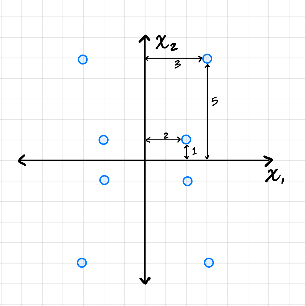
Suppose PCA is used to reduce the dimensionality of the centered data shown below from 2 dimensions to 1.
Part 1)
What will be the reconstruction error?
Solution
\(52\).
The first thing to figure out is what the first principal component (first eigenvector of the covariance matrix) is, since this is the direction onto which the data will be projected. Remember that the first eigenvector points in the direction of maximum variance, and in this plot that appears to be straight up (or down). Thus, the first principal component is \((0, 1)^T\)(or \((0, -1)^T\)).
Next, we imagine projecting all of the data onto this line. Since the first eigenvector is vertical, all of the data is projected onto the \(x_2\)-axis. In the process, every point's \(x_1\)-coordinate is lost, and becomes zero, while the \(x_2\)-coordinate remains unchanged. The figure below shows these projected points in red (note that each red point is actually two points on top of each other, since both \((x_1, x_2)^T\) and \((-x_1, x_2)^T\) project to \((0, x_2)^T\)).
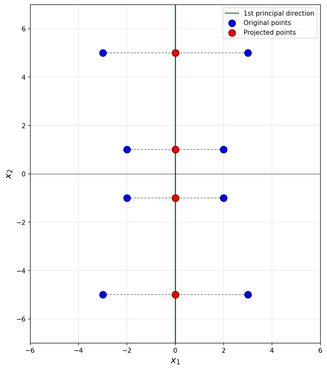
To compute the reconstruction error, we find the squared distance between each point's original position and its projected position. Starting with the upper-right-most point at \((3, 5)^T\), its projection is \((0, 5)^T\), and the squared distance between these two points is \((3 - 0)^2 + (5 - 5)^2 = 9\). For the point at \((2, 1)^T\), its projection is \((0, 1)^T\), and the squared distance is \((2 - 0)^2 + (1 - 1)^2 = 4\).
We could continue, manually calculating the squared distance for each point, but the symmetry of the data allows us to be more efficient. There are four points in the data set that are exactly like the first we just considered and which will have a reconstruction error of 9 each. Similarly, there are four points like the second we considered, each with a reconstruction error of 4. Therefore, the total reconstruction error is:
Part 2)
What is the smallest eigenvalue of the data's covariance matrix?
Solution
\(13/2\).
Remember that the smallest eigenvalue of the data's covariance matrix is equal to the variance of the second PCA feature. That is, it is the variance in the direction of the second principal component (the second eigenvector of the covariance matrix), which in this case is the vector \((1, 0)^T\)(or \((-1, 0)^T\)).
The variance of the data in this direction can be computed by
where \(x_i\) is the \(x_1\)-coordinate of the \(i\)-th data point, \(\mu\) is the mean of all the \(x_1\)-coordinates, and \(n\) is the number of data points. Since hte data is centered, \(\mu = 0\). Therefore, we just need to compute the average of the squared \(x_1\)-coordinates.
Reading these off, we have four points whose \(x_1\)-coordinate is \(3\) or \(-3\), and four points whose \(x_1\)-coordinate is \(2\) or \(-2\). So the variance is:
Therefore, the smallest eigenvalue of the data's covariance matrix is \(13/2\).
Problem #087
Tags: pca, covariance, eigenvalues, lecture-07, quiz-04
Consider the centered data set shown below. The data is symmetric across both axes.
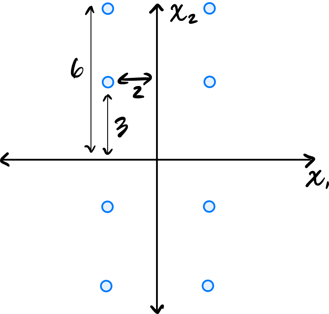
Let \(C\) be the empirical covariance matrix. What is the largest eigenvalue of \(C\)?
Solution
\(45/2\).
Remember that the largest eigenvalue of the data's covariance matrix is equal to the variance of the first PCA feature. That is, it is the variance in the direction of the first principal component (the first eigenvector of the covariance matrix).
Since the data is symmetric across both axes, the eigenvectors of the covariance matrix are aligned with the coordinate axes. From the figure, the data is more spread out vertically than horizontally, so the first principal component is the vector \((0, 1)^T\)(or \((0, -1)^T\)).
The variance of the data in this direction can be computed by
where \(x_i\) is the \(x_2\)-coordinate of the \(i\)-th data point, \(\mu\) is the mean of all the \(x_2\)-coordinates, and \(n\) is the number of data points. Since the data is centered, \(\mu = 0\). Therefore, we just need to compute the average of the squared \(x_2\)-coordinates.
Reading these off, we have four points whose \(x_2\)-coordinate is \(6\) or \(-6\), and four points whose \(x_2\)-coordinate is \(3\) or \(-3\). So the variance is:
Therefore, the largest eigenvalue of the data's covariance matrix is \(45/2\).
Problem #088
Tags: lecture-07, eigenvalues, variance, pca
Let \(\mathcal X = \{\vec{x}^{(1)}, \ldots, \vec{x}^{(100)}\}\) be a set of 100 points in \(3\) dimensions. The variance in the direction of \(\hat{e}^{(1)}\) is 20, the variance in the direction of \(\hat{e}^{(2)}\) is 12, and the variance in the direction of \(\hat{e}^{(3)}\) is 10.
Suppose PCA is performed, but dimensionality is not reduced; that is, each point \(\vec{x}^{(i)}\) is transformed to the vector \(\vec{z}^{(i)} = U \vec{x}^{(i)}\), where \(U\) is a matrix whose \(3\) rows are the (orthonormal) eigenvectors of the data covariance matrix. Let \(\mathcal Z = \{\vec{z}^{(1)}, \ldots, \vec{z}^{(100)}\}\) be the resulting data set.
Suppose \(C\) is the covariance matrix of the new data set, \(\mathcal Z\), and that the top two eigenvalues of \(C\) are 25 and 15. What is the third eigenvalue?
Solution
\(2\).
Although it wasn't discussed in lecture, it turns out that the total variance is preserved under orthogonal transformations. The total variance of the original data is:
After PCA, the covariance matrix \(C\) of \(\mathcal Z\) is diagonal with the eigenvalues on the diagonal. The sum of eigenvalues equals the total variance:
Problem #089
Tags: reconstruction error, pca, covariance, eigenvalues, lecture-07, quiz-04
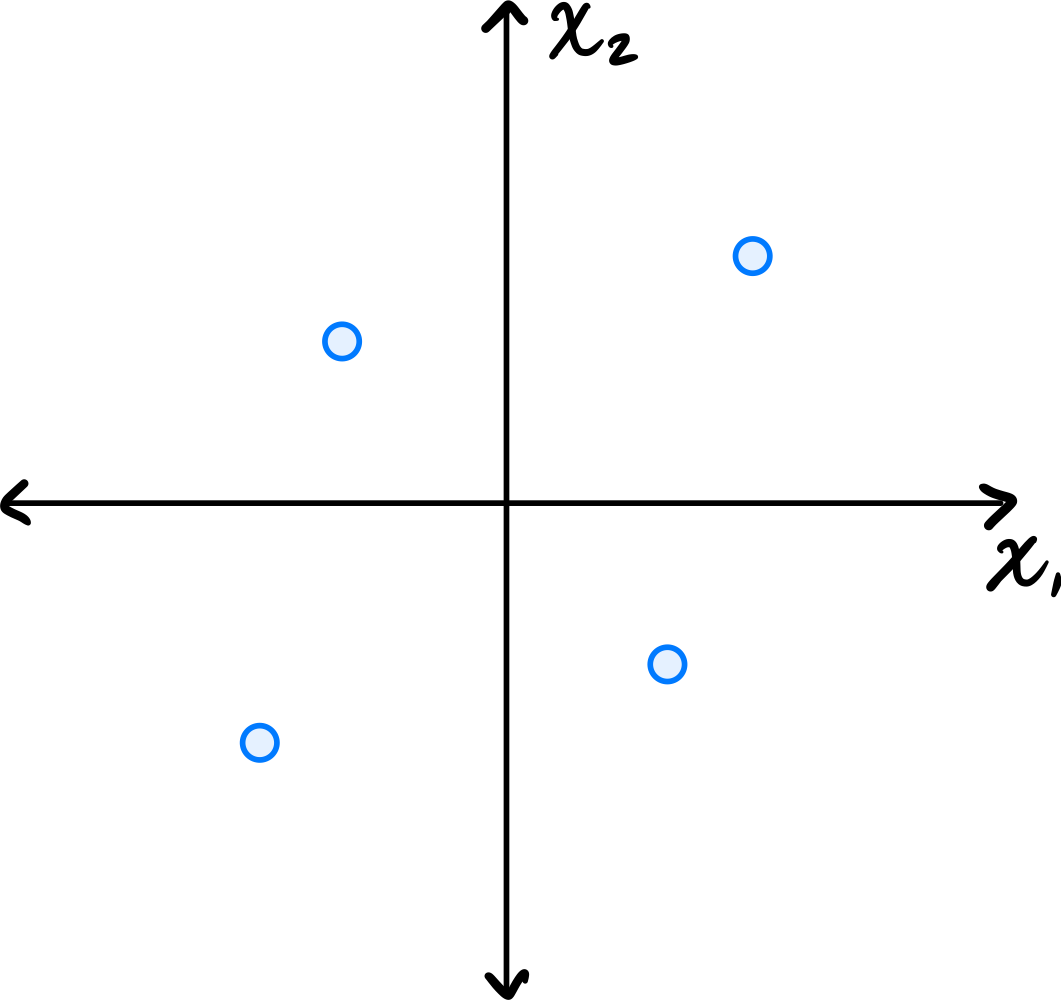
Consider the centered data set consisting of four points:
Suppose PCA is used to reduce the dimensionality of the data from 2 dimensions to 1.
Part 1)
What will be the reconstruction error?
Solution
\(16\).
The first thing to figure out is what the first principal component (first eigenvector of the covariance matrix) is, since this is the direction onto which the data will be projected. Remember that the first eigenvector points in the direction of maximum variance. Looking at the data, the points \((3, 3)^T\) and \((-3, -3)^T\) are farther from the origin than the points \((-2, 2)^T\) and \((2, -2)^T\), so the direction of maximum variance is along the line \(x_2 = x_1\). Thus, the first principal component is \(\frac{1}{\sqrt{2}}(1, 1)^T\)(or \(\frac{1}{\sqrt{2}}(-1, -1)^T\)).
Next, we imagine projecting all of the data onto this line. The figure below shows these projected points in red.
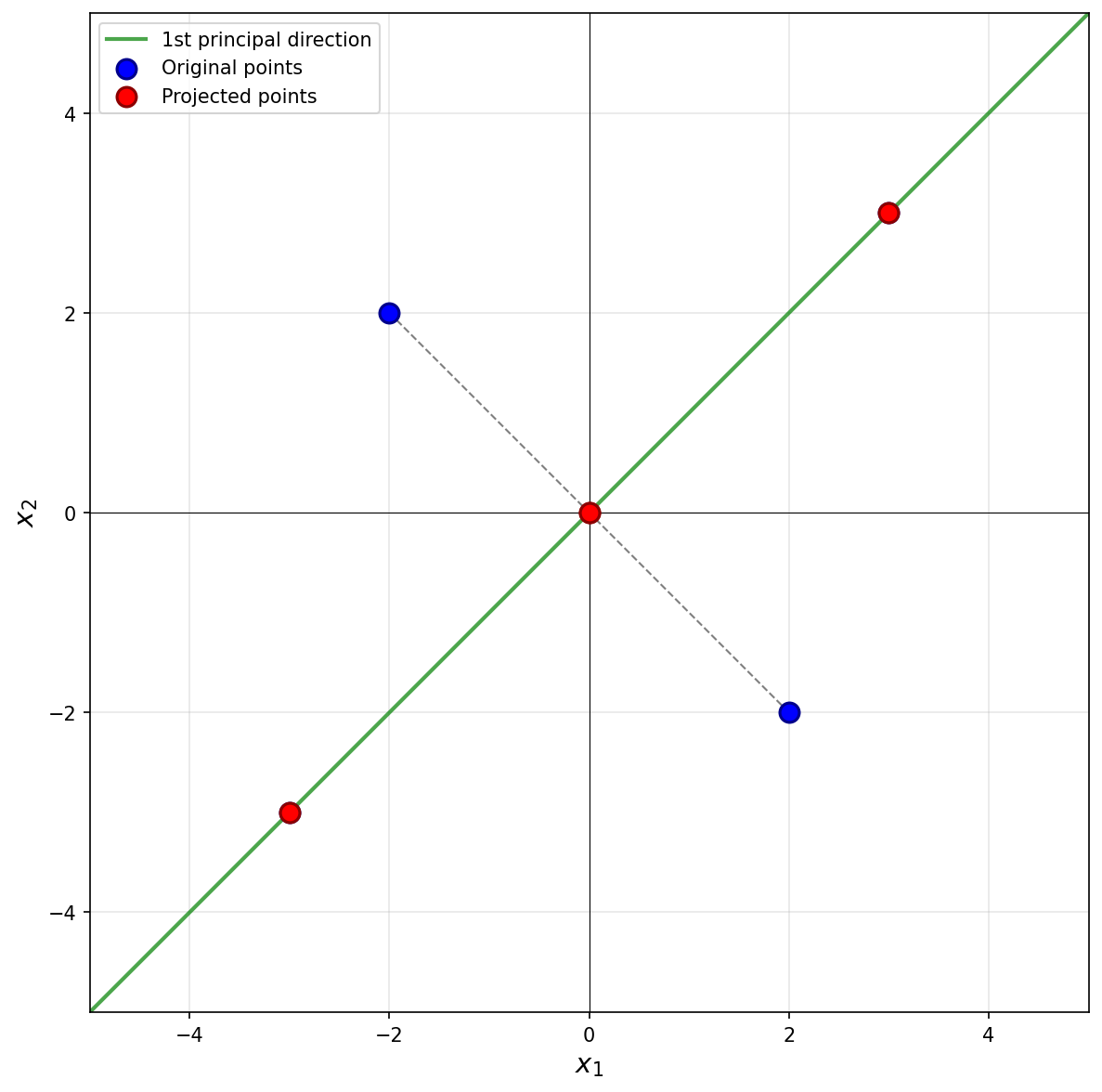
Notice that the points \((3, 3)^T\) and \((-3, -3)^T\) already lie on the line \(x_2 = x_1\), so they project to themselves. Their reconstruction error is zero. The points \((-2, 2)^T\) and \((2, -2)^T\) lie on the line \(x_2 = -x_1\), which is perpendicular to the first principal component. These points both project to the origin \((0, 0)^T\).
To compute the reconstruction error, we find the squared distance between each point's original position and its projected position. For the point at \((-2, 2)^T\), its projection is \((0, 0)^T\), and the squared distance is \((-2 - 0)^2 + (2 - 0)^2 = 4 + 4 = 8\). Similarly, the point \((2, -2)^T\) projects to \((0, 0)^T\) with squared distance \(8\).
Therefore, the total reconstruction error is:
Part 2)
What is the smallest eigenvalue of the data's covariance matrix?
Solution
\(4\).
Remember that the smallest eigenvalue of the data's covariance matrix is equal to the variance of the second PCA feature.
The second PCA feature corresponds to each point's projection onto the second principal component (the second eigenvector of the covariance matrix, and the dashed line in the figure above). In this case, we see that two of the points, \((3, 3)^T\) and \((-3, -3)^T\), project to the origin \((0, 0)^T\), and will have a second PCA feature value of \(0\). The other two points are at \(8\) units away from the origin along this direction, so their second PCA feature values are \(2 \sqrt{2}\) and \(-2 \sqrt{2}\). You could also project these points onto the second principal component to verify this:
Therefore, the second PCA feature values for the four points are 0, 0, 2, and -2. The variance of these (centered) values is:
Problem #097
Tags: lecture-08, laplacian eigenmaps, quiz-05, eigenvalues, eigenvectors
Given a \(4 \times 4\) Graph Laplacian matrix \(L\), the 4 (eigenvalue, eigenvector) pairs of this matrix are given as \((3, \vec v_1)\), \((0, \vec v_2)\), \((8, \vec v_3)\), \((14, \vec v_4)\).
You need to pick one eigenvector. Which of the above eigenvectors will be a non-trivial solution to the spectral embedding problem?
Solution
\(\vec v_1\).
The embedding is the eigenvector with the smallest eigenvalue that is strictly greater than \(0\). The eigenvector \(\vec v_2\) corresponds to eigenvalue \(0\), which gives the trivial solution (all embeddings equal). Among the remaining eigenvectors, \(\vec v_1\) has the smallest eigenvalue (\(3\)), so it is the non-trivial solution to the spectral embedding problem.