Problems tagged with "eigenvectors"
Problem #028
Tags: linear algebra, quiz-03, eigenvalues, eigenvectors, lecture-04
Let \(A = \begin{pmatrix} 3 & 1 \\ 1 & 3 \end{pmatrix}\) and let \(\vec v = (1, 1)^T\).
True or False: \(\vec v\) is an eigenvector of \(A\). If true, what is the corresponding eigenvalue?
Solution
True, with eigenvalue \(\lambda = 4\).
We compute:
Since \(A \vec v = 4 \vec v\), the vector \(\vec v\) is an eigenvector with eigenvalue \(4\).
Problem #029
Tags: linear algebra, quiz-03, eigenvalues, eigenvectors, lecture-04
Let \(A = \begin{pmatrix} 2 & 1 \\ 1 & 2 \end{pmatrix}\) and let \(\vec v = (1, 2)^T\).
True or False: \(\vec v\) is an eigenvector of \(A\). If true, what is the corresponding eigenvalue?
Solution
False.
We compute:
For \(\vec v\) to be an eigenvector, we would need \(A \vec v = \lambda\vec v\) for some scalar \(\lambda\). This would require:
From the first component, we would need \(\lambda = 4\). From the second component, we would need \(\lambda = \frac{5}{2}\). Since these two values are not equal, there is no such \(\lambda\) that satisfies both equations. Therefore, \(\vec v\) is not an eigenvector of \(A\).
Problem #030
Tags: linear algebra, quiz-03, eigenvalues, eigenvectors, lecture-04
Let \(A = \begin{pmatrix} 1 & 1 & 3 \\ 1 & 2 & 1 \\ 3 & 1 & 9 \end{pmatrix}\) and let \(\vec v = (1, 4, -1)^T\).
True or False: \(\vec v\) is an eigenvector of \(A\). If true, what is the corresponding eigenvalue?
Solution
True, with eigenvalue \(\lambda = 2\).
We compute:
Since \(A \vec v = 2 \vec v\), the vector \(\vec v\) is an eigenvector with eigenvalue \(2\).
Problem #031
Tags: linear algebra, quiz-03, eigenvalues, eigenvectors, lecture-04
Let \(A = \begin{pmatrix} 5 & 1 & 1 & 1 \\ 1 & 5 & 1 & 1 \\ 1 & 1 & 5 & 1 \\ 1 & 1 & 1 & 5 \end{pmatrix}\) and let \(\vec v = (1, 2, -2, -1)^T\).
True or False: \(\vec v\) is an eigenvector of \(A\). If true, what is the corresponding eigenvalue?
Solution
True, with eigenvalue \(\lambda = 4\).
We compute:
Since \(A \vec v = 4 \vec v\), the vector \(\vec v\) is an eigenvector with eigenvalue \(4\).
Problem #032
Tags: linear algebra, quiz-03, eigenvalues, eigenvectors, lecture-04
Let \(A = \begin{pmatrix} 1 & 6 \\ 6 & 6 \end{pmatrix}\) and let \(\vec v = (3, -2)^T\).
True or False: \(\vec v\) is an eigenvector of \(A\). If true, what is the corresponding eigenvalue?
Solution
True, with eigenvalue \(\lambda = -3\).
We compute:
Since \(A \vec v = -3 \vec v\), the vector \(\vec v\) is an eigenvector with eigenvalue \(-3\).
Problem #033
Tags: linear algebra, quiz-03, eigenvalues, eigenvectors, lecture-04
Let \(\vec v\) be a unit vector in \(\mathbb R^d\), and let \(I\) be the \(d \times d\) identity matrix. Consider the matrix \(P\) defined as:
True or False: \(\vec v\) is an eigenvector of \(P\).
Solution
True.
To verify this, we compute \(P \vec v\):
Since \(P \vec v = -\vec v = (-1) \vec v\), we see that \(\vec v\) is an eigenvector of \(P\) with eigenvalue \(-1\).
Note: The matrix \(P = I - 2 \vec v \vec v^T\) is called a Householder reflection matrix, which reflects vectors across the hyperplane orthogonal to \(\vec v\).
Problem #034
Tags: linear algebra, quiz-03, eigenvalues, eigenvectors, lecture-04
Let \(A\) be the matrix:
It can be verified that the vector \(\vec{u}^{(1)} = (2, 1)^T\) is an eigenvector of \(A\).
Part 1)
What is the eigenvalue associated with \(\vec{u}^{(1)}\)?
Solution
The eigenvalue is \(\lambda_1 = 6\).
To find the eigenvalue, we compute \(A \vec{u}^{(1)}\):
Therefore, \(\lambda_1 = 6\).
Part 2)
Find another eigenvector \(\vec{u}^{(2)}\) of \(A\). Your eigenvector should have an eigenvalue that is different from \(\vec{u}^{(1)}\)'s eigenvalue. It does not need to be normalized.
Solution
\(\vec{u}^{(2)} = (1, -2)^T\)(or any scalar multiple).
Since \(A\) is symmetric, we know that we can always find two orthogonal eigenvectors. This suggests that we should find a vector orthogonal to \(\vec{u}^{(1)} = (2, 1)^T\) and make sure that it is indeed an eigenvector.
We know from the math review in Week 01 that the vector \((1, -2)^T\) is orthogonal to \((2, 1)^T\)(in general, \((a, b)^T\) is orthogonal to \((-b, a)^T\)).
We can verify:
So the eigenvalue is \(\lambda_2 = 1\), which is indeed different from \(\lambda_1 = 6\).
Problem #035
Tags: linear algebra, quiz-03, eigenvalues, eigenvectors, lecture-04
Let \(D\) be the diagonal matrix:
Part 1)
What is the top eigenvalue of \(D\)? What eigenvector corresponds to this eigenvalue?
Solution
The top eigenvalue is \(7\).
For a diagonal matrix, the eigenvalues are exactly the diagonal entries. The diagonal entries are \(2, -5, 7\), and the largest is \(7\).
An eigenvector corresponding to this eigenvalue is \(\vec v = (0, 0, 1)^T\).
Part 2)
What is the bottom (smallest) eigenvalue of \(D\)? What eigenvector corresponds to this eigenvalue?
Solution
The bottom eigenvalue is \(-5\).
An eigenvector corresponding to this eigenvalue is \(\vec w = (0, 1, 0)^T\).
Problem #036
Tags: linear algebra, quiz-03, eigenvalues, eigenvectors, lecture-04, linear transformations
Consider the linear transformation \(\vec f : \mathbb{R}^2 \to\mathbb{R}^2\) that reflects vectors over the line \(y = -x\).
Find two orthogonal eigenvectors of this transformation and their corresponding eigenvalues.
Solution
The eigenvectors are \((1, -1)^T\) with \(\lambda = 1\), and \((1, 1)^T\) with \(\lambda = -1\).
Geometrically, vectors along the line \(y = -x\)(i.e., multiples of \((1, -1)^T\)) are unchanged by reflection over that line, so they have eigenvalue \(1\). Vectors perpendicular to the line \(y = -x\)(i.e., multiples of \((1, 1)^T\)) are flipped to point in the opposite direction, so they have eigenvalue \(-1\).
Problem #037
Tags: linear algebra, quiz-03, eigenvalues, eigenvectors, lecture-04, linear transformations
Consider the linear transformation \(\vec f : \mathbb{R}^2 \to\mathbb{R}^2\) that scales vectors along the line \(y = x\) by a factor of 2, and scales vectors along the line \(y = -x\) by a factor of 3.
Find two orthogonal eigenvectors of this transformation and their corresponding eigenvalues.
Solution
The eigenvectors are \((1, 1)^T\) with \(\lambda = 2\), and \((1, -1)^T\) with \(\lambda = 3\).
Geometrically, vectors along the line \(y = x\)(i.e., multiples of \((1, 1)^T\)) are scaled by a factor of 2, so they have eigenvalue \(2\). Vectors along the line \(y = -x\)(i.e., multiples of \((1, -1)^T\)) are scaled by a factor of 3, so they have eigenvalue \(3\).
Problem #038
Tags: linear algebra, quiz-03, eigenvalues, eigenvectors, lecture-04, linear transformations
Consider the linear transformation \(\vec f : \mathbb{R}^2 \to\mathbb{R}^2\) that rotates vectors by \(180°\).
Find two orthogonal eigenvectors of this transformation and their corresponding eigenvalues.
Solution
Any pair of orthogonal vectors works, such as \((1, 0)^T\) and \((0, 1)^T\). Both have eigenvalue \(\lambda = -1\).
Geometrically, rotating any vector by \(180°\) reverses its direction, so \(\vec f(\vec v) = -\vec v\) for all \(\vec v\). This means every nonzero vector is an eigenvector with eigenvalue \(-1\).
Since we need two orthogonal eigenvectors, any orthogonal pair will do.
Problem #039
Tags: linear algebra, quiz-03, eigenvalues, eigenvectors, lecture-04
Consider the diagonal matrix:
How many unit length eigenvectors does \(A\) have?
Solution
\(\infty\) The upper-left \(2 \times 2\) block of \(A\) is the identity matrix. Recall from lecture that the identity matrix has infinitely many eigenvectors: every nonzero vector is an eigenvector of the identity with eigenvalue 1.
Similarly, any vector of the form \((a, b, 0)^T\) where \(a\) and \(b\) are not both zero satisfies:
So any such vector is an eigenvector with eigenvalue 1. There are infinitely many unit vectors of this form (they form a circle in the \(x\)-\(y\) plane), so \(A\) has infinitely many unit length eigenvectors.
Additionally, \((0, 0, 1)^T\) is an eigenvector with eigenvalue 5.
Problem #040
Tags: linear algebra, quiz-03, spectral theorem, eigenvectors, lecture-04
Consider the matrix:
True or False: The spectral theorem guarantees that \(A\) has 2 orthogonal eigenvectors.
Solution
False.
The spectral theorem only applies to symmetric matrices. The matrix \(A\) is not symmetric because \(A^T \neq A\):
Since \(A\) is not symmetric, the spectral theorem does not apply, and we cannot use it to conclude anything about \(A\)'s eigenvectors.
Problem #041
Tags: linear algebra, quiz-03, spectral theorem, eigenvectors, lecture-04
Suppose \(A\) is a symmetric matrix, and \(\vec{u}^{(1)}\) and \(\vec{u}^{(2)}\) are both eigenvectors of \(A\).
True or False: \(\vec{u}^{(1)}\) and \(\vec{u}^{(2)}\) must be orthogonal.
Solution
False.
Consider the identity matrix \(I\). Every nonzero vector is an eigenvector of \(I\) with eigenvalue 1. For example, both \((1, 0)^T\) and \((1, 1)^T\) are eigenvectors of \(I\), but they are not orthogonal:
The spectral theorem says that you can find\(n\) orthogonal eigenvectors for an \(n \times n\) symmetric matrix, but it does not say that every pair of eigenvectors is orthogonal.
Aside: It can be shown that if \(\vec{u}^{(1)}\) and \(\vec{u}^{(2)}\) have different eigenvalues, then they must be orthogonal.
Problem #042
Tags: linear algebra, quiz-03, spectral theorem, eigenvectors, diagonalization, lecture-04
Suppose \(A\) is a \(d \times d\) symmetric matrix.
True or False: There exists an orthonormal basis in which \(A\) is diagonal.
Solution
True.
By the spectral theorem, every \(d \times d\) symmetric matrix has \(d\) mutually orthogonal eigenvectors. If we normalize these eigenvectors, they form an orthonormal basis.
In this eigenbasis, the matrix \(A\) is diagonal: the diagonal entries are the eigenvalues of \(A\).
Problem #043
Tags: linear algebra, quiz-03, symmetric matrices, eigenvectors, lecture-04, linear transformations
The figure below shows a linear transformation \(\vec{f}\) applied to points on the unit circle. Each arrow shows the direction and relative magnitude of \(\vec{f}(\vec{x})\) for a point \(\vec{x}\) on the circle.
True or False: The linear transformation \(\vec{f}\) is symmetric.
Solution
False.
Recall from lecture that symmetric linear transformations have orthogonal axes of symmetry. In the visualization, this would appear as two perpendicular directions where the arrows point directly outward (or inward) from the circle.
In this figure, there are no such orthogonal axes of symmetry. The pattern of arrows does not exhibit the characteristic symmetry of a symmetric transformation.
Problem #044
Tags: linear algebra, quiz-03, diagonal matrices, eigenvectors, lecture-04, linear transformations
The figure below shows a linear transformation \(\vec{f}\) applied to points on the unit circle. Each arrow shows the direction and relative magnitude of \(\vec{f}(\vec{x})\) for a point \(\vec{x}\) on the circle.
True or False: The matrix representing \(\vec{f}\) with respect to the standard basis is diagonal.
Solution
True.
A matrix is diagonal if and only if the standard basis vectors are eigenvectors. In the visualization, eigenvectors correspond to directions where the arrows point radially (directly outward or inward).
Looking at the figure, the arrows at \((1, 0)\) and \((-1, 0)\) point horizontally, and the arrows at \((0, 1)\) and \((0, -1)\) point vertically. This means the standard basis vectors \(\hat e^{(1)} = (1, 0)^T\) and \(\hat e^{(2)} = (0, 1)^T\) are eigenvectors.
Since the standard basis vectors are eigenvectors, the matrix is diagonal in the standard basis.
Problem #045
Tags: linear algebra, eigenbasis, quiz-03, eigenvalues, eigenvectors, lecture-04
Let \(\vec{u}^{(1)}, \vec{u}^{(2)}, \vec{u}^{(3)}\) be three unit length orthonormal eigenvectors of a linear transformation \(\vec{f}\), with eigenvalues \(8\), \(4\), and \(-3\) respectively.
Suppose a vector \(\vec{x}\) can be written as:
What is \(\vec{f}(\vec{x})\), expressed in coordinates with respect to the eigenbasis \(\{\vec{u}^{(1)}, \vec{u}^{(2)}, \vec{u}^{(3)}\}\)?
Solution
\([\vec{f}(\vec{x})]_{\mathcal{U}} = (16, -12, -3)^T\) Using linearity and the eigenvector property:
Since \(\vec{u}^{(1)}\) is an eigenvector with eigenvalue \(8\), we have \(\vec{f}(\vec{u}^{(1)}) = 8\vec{u}^{(1)}\). Similarly, \(\vec{f}(\vec{u}^{(2)}) = 4\vec{u}^{(2)}\) and \(\vec{f}(\vec{u}^{(3)}) = -3\vec{u}^{(3)}\):
In the eigenbasis, this is simply \((16, -12, -3)^T\).
Problem #046
Tags: linear algebra, eigenbasis, quiz-03, eigenvalues, eigenvectors, lecture-04
Let \(\vec{u}^{(1)}, \vec{u}^{(2)}, \vec{u}^{(3)}\) be three unit length orthonormal eigenvectors of a linear transformation \(\vec{f}\), with eigenvalues \(5\), \(-2\), and \(3\) respectively.
Suppose a vector \(\vec{x}\) can be written as:
What is \(\vec{f}(\vec{x})\), expressed in coordinates with respect to the eigenbasis \(\{\vec{u}^{(1)}, \vec{u}^{(2)}, \vec{u}^{(3)}\}\)?
Solution
\([\vec{f}(\vec{x})]_{\mathcal{U}} = (20, -2, -6)^T\) Using linearity and the eigenvector property:
Since \(\vec{u}^{(1)}\) is an eigenvector with eigenvalue \(5\), we have \(\vec{f}(\vec{u}^{(1)}) = 5\vec{u}^{(1)}\). Similarly, \(\vec{f}(\vec{u}^{(2)}) = -2\vec{u}^{(2)}\) and \(\vec{f}(\vec{u}^{(3)}) = 3\vec{u}^{(3)}\):
In the eigenbasis, this is simply \((20, -2, -6)^T\).
Problem #047
Tags: optimization, linear algebra, quiz-03, eigenvalues, eigenvectors, lecture-04
Let \(A\) be a symmetric matrix with eigenvalues \(6\) and \(-9\).
True or False: The maximum value of \(\|A\vec{x}\|\) over all unit vectors \(\vec{x}\) is \(6\).
Solution
False. The maximum is \(9\).
The maximum of \(\|A\vec{x}\|\) over unit vectors is achieved when \(\vec{x}\) is an eigenvector corresponding to the eigenvalue with the largest absolute value.
Here, \(|-9| = 9 > 6 = |6|\), so the maximum is achieved at the eigenvector with eigenvalue \(-9\).
If \(\vec{u}\) is a unit eigenvector with eigenvalue \(-9\), then:
Problem #048
Tags: optimization, linear algebra, quiz-03, eigenvalues, eigenvectors, quadratic forms, lecture-04
Let \(A\) be a \(3 \times 3\) symmetric matrix with the following eigenvectors and corresponding eigenvalues: \(\vec{u}^{(1)} = \frac{1}{3}(1, 2, 2)^T\) has eigenvalue \(4\), \(\vec{u}^{(2)} = \frac{1}{3}(2, 1, -2)^T\) has eigenvalue \(1\), and \(\vec{u}^{(3)} = \frac{1}{3}(2, -2, 1)^T\) has eigenvalue \(-10\).
Consider the quadratic form \(\vec{x}\cdot A\vec{x}\).
Part 1)
What unit vector \(\vec{x}\) maximizes \(\vec{x}\cdot A\vec{x}\)?
Solution
\(\vec{u}^{(1)} = \frac{1}{3}(1, 2, 2)^T\) The quadratic form \(\vec{x}\cdot A\vec{x}\) is maximized by the eigenvector with the largest eigenvalue. Among \(4\), \(1\), and \(-10\), the largest is \(4\), so the maximizer is \(\vec{u}^{(1)}\).
Part 2)
What is the maximum value of \(\vec{x}\cdot A\vec{x}\) over all unit vectors?
Solution
\(4\) The maximum value equals the largest eigenvalue. We can verify:
Part 3)
What unit vector \(\vec{x}\) minimizes \(\vec{x}\cdot A\vec{x}\)?
Solution
\(\vec{u}^{(3)} = \frac{1}{3}(2, -2, 1)^T\) The quadratic form is minimized by the eigenvector with the smallest eigenvalue. Among \(4\), \(1\), and \(-10\), the smallest is \(-10\), so the minimizer is \(\vec{u}^{(3)}\).
Part 4)
What is the minimum value of \(\vec{x}\cdot A\vec{x}\) over all unit vectors?
Solution
\(-10\) The minimum value equals the smallest eigenvalue. We can verify:
Problem #049
Tags: linear algebra, quiz-03, eigenvalues, eigenvectors, lecture-04
Let \(A\) be a symmetric matrix with top eigenvalue \(\lambda\). Let \(B = A + 5I\), where \(I\) is the identity matrix.
True or False: The top eigenvalue of \(B\) must be \(\lambda + 5\).
Solution
True.
The main thing to realize is that \(A\) and \(B\) have the same eigenvectors. If \(\vec v\) is an eigenvector of \(A\) with eigenvalue \(\lambda\), then:
Thus, \(\vec v\) is also an eigenvector of \(B\) with eigenvalue \(\lambda + 5\).
This means that the eigenvalues of \(B\) are simply the eigenvalues of \(A\) shifted by 5. Therefore, if \(\lambda\) is the top eigenvalue of \(A\), then \(\lambda + 5\) is the top eigenvalue of \(B\).
Problem #053
Tags: linear algebra, quiz-03, lecture-05, eigenvalues, eigenvectors, diagonalization
Let \(\vec f\) be a linear transformation with eigenvectors and eigenvalues:
What is \(\vec f(\vec x)\) for \(\vec x = (3, 1)^T\)?
Solution
\(\vec f(\vec x) = (3, 5)^T\).
We'll take the three step approach of 1) finding the coordinates of \(\vec x\) in the eigenbasis, 2) applying the transformation in that basis (where the matrix of the transformation \(A_\mathcal{U}\) is diagonal and consists of the eigenvalues), and 3) converting back to the standard basis.
We saw in lecture that we can do this all in one go using the change of basis matrix \(U\):
where \(U\) is the change of basis matrix with the eigenvectors as rows and \(A_\mathcal{U}\) is the diagonal matrix with the eigenvalues on the diagonal. In this case, they are:
Then:
Problem #054
Tags: linear algebra, quiz-03, lecture-05, eigenvalues, eigenvectors, diagonalization
Let \(\vec f\) be a linear transformation with eigenvectors and eigenvalues:
What is \(\vec f(\vec x)\) for \(\vec x = (1, 1, 2)^T\)?
Solution
\(\vec f(\vec x) = (3, 3, 2)^T\).
We'll take the three step approach of 1) finding the coordinates of \(\vec x\) in the eigenbasis, 2) applying the transformation in that basis (where the matrix of the transformation \(A_\mathcal{U}\) is diagonal and consists of the eigenvalues), and 3) converting back to the standard basis.
We saw in lecture that we can do this all in one go using the change of basis matrix \(U\):
where \(U\) is the change of basis matrix with the eigenvectors as rows and \(A_\mathcal{U}\) is the diagonal matrix with the eigenvalues on the diagonal. In this case, they are:
Then:
Problem #055
Tags: linear algebra, quiz-03, lecture-05, eigenvalues, eigenvectors, diagonalization
Let \(\vec f\) be a linear transformation with eigenvectors and eigenvalues:
What is \(\vec f(\vec x)\) for \(\vec x = (4, 0, 0, 0)^T\)?
Solution
\(\vec f(\vec x) = (7, 5, 3, 1)^T\).
We'll take the three step approach of 1) finding the coordinates of \(\vec x\) in the eigenbasis, 2) applying the transformation in that basis (where the matrix of the transformation \(A_\mathcal{U}\) is diagonal and consists of the eigenvalues), and 3) converting back to the standard basis.
We saw in lecture that we can do this all in one go using the change of basis matrix \(U\):
where \(U\) is the change of basis matrix with the eigenvectors as rows and \(A_\mathcal{U}\) is the diagonal matrix with the eigenvalues on the diagonal. In this case, they are:
Then:
Problem #056
Tags: linear algebra, quiz-03, symmetric matrices, spectral theorem, eigenvalues, eigenvectors, lecture-05
Find a symmetric \(2 \times 2\) matrix \(A\) whose eigenvectors are \(\hat{u}^{(1)} = \frac{1}{\sqrt{5}}(1, 2)^T\) with eigenvalue \(6\) and \(\hat{u}^{(2)} = \frac{1}{\sqrt{5}}(2, -1)^T\) with eigenvalue \(1\).
Solution
\(A = \begin{pmatrix} 2 & 2 \\ 2 & 5 \end{pmatrix}\).
We saw in lecture that a symmetric matrix \(A\) can be written as \(A = U^T \Lambda U\), where \(U\) is the matrix whose rows are the eigenvectors of \(A\) and \(\Lambda\) is the diagonal matrix of eigenvalues.
This means that if we know the eigenvectors and eigenvalues of a symmetric matrix, we can "work backwards" to find the matrix itself.
In this case:
Therefore:
Problem #057
Tags: linear algebra, quiz-03, symmetric matrices, spectral theorem, eigenvalues, eigenvectors, lecture-05
Find a symmetric \(3 \times 3\) matrix \(A\) whose eigenvectors are \(\hat{u}^{(1)} = \frac{1}{3}(1, 2, 2)^T\) with eigenvalue \(9\), \(\hat{u}^{(2)} = \frac{1}{3}(2, 1, -2)^T\) with eigenvalue \(18\), and \(\hat{u}^{(3)} = \frac{1}{3}(2, -2, 1)^T\) with eigenvalue \(-9\).
Solution
\(A = \begin{pmatrix} 5 & 10 & -8 \\ 10 & 2 & 2 \\ -8 & 2 & 11 \end{pmatrix}\).
We saw in lecture that a symmetric matrix \(A\) can be written as \(A = U^T \Lambda U\), where \(U\) is the matrix whose rows are the eigenvectors of \(A\) and \(\Lambda\) is the diagonal matrix of eigenvalues.
In this case:
Therefore:
Problem #068
Tags: covariance, eigenvectors, quiz-04, variance, lecture-06
Let \(C\) be the sample covariance matrix of a centered data set, and suppose \(\vec{u}^{(1)}, \vec{u}^{(2)}, \vec{u}^{(3)}\) are normalized eigenvectors of \(C\) with eigenvalues \(\lambda_1 = 9, \lambda_2 = 3, \lambda_3=0\), respectively.
Suppose \(\vec x = \frac{1}{\sqrt 2}\vec{u}^{(1)} + \frac{1}{\sqrt 6}\vec{u}^{(2)} + \frac{1}{\sqrt 3}\vec{u}^{(3)}\). What is the variance in the direction of \(\vec x\)?
Solution
\(5\) Remember that for any unit vector \(\vec u\), the variance in the direction of \(\vec u\) is given by \(\vec u^T C \vec u\). So, for the vector \(\vec x\), we have
Since \(\vec{u}^{(1)}, \vec{u}^{(2)}, \vec{u}^{(3)}\) are eigenvectors of \(C\), the matrix multiplication simplifies:
Problem #070
Tags: lecture-06, quiz-04, eigenvectors, pca
Consider the data set shown below:
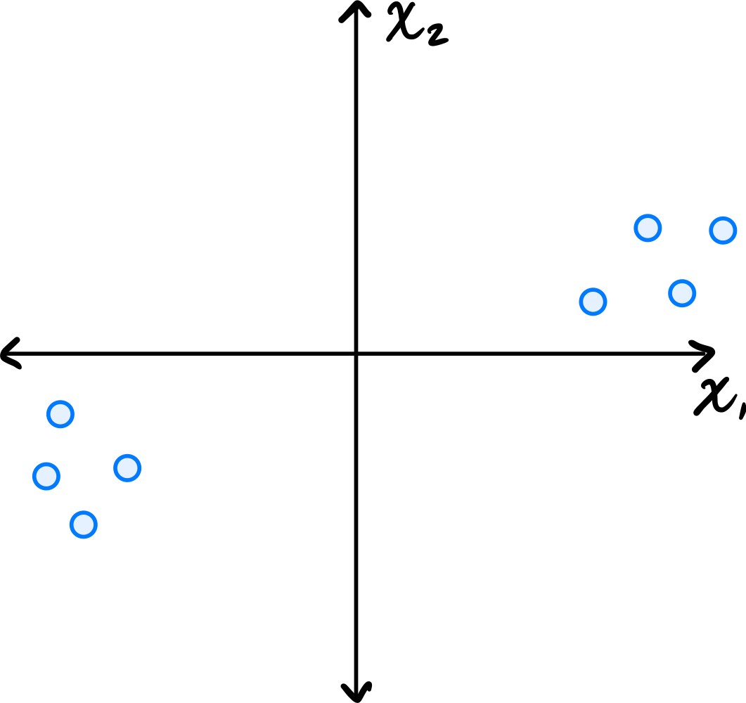
Which of the following could possibly be the top eigenvector of the data's sample covariance matrix?
Solution
\((3, 1)^T\) The top eigenvector of the covariance matrix points in the direction of greatest variance. Looking at the scatter plot, the data is elongated along a direction that has a positive slope, rising more in the \(x_1\) direction than the \(x_2\) direction. The vector \((3, 1)^T\) points roughly in this direction.
\((1, 0)^T\) and \((0, 1)^T\) are along the axes, which don't align with the data's elongation. \((1, 1)^T\) has too steep a slope compared to the apparent direction of the data.
Problem #073
Tags: covariance, eigenvectors, quiz-04, variance, lecture-06
Let \(C\) be the sample covariance matrix of a centered data set, and suppose \(\vec{u}^{(1)}, \vec{u}^{(2)}, \vec{u}^{(3)}\) are normalized eigenvectors of \(C\) with eigenvalues \(\lambda_1 = 16, \lambda_2 = 12, \lambda_3=0\), respectively.
Suppose \(\vec x = \frac{1}{\sqrt 2}\vec{u}^{(1)} + \frac{1}{\sqrt 6}\vec{u}^{(2)} + \frac{1}{\sqrt 3}\vec{u}^{(3)}\). What is the variance in the direction of \(\vec x\)?
Solution
\(10\) Remember that for any unit vector \(\vec u\), the variance in the direction of \(\vec u\) is given by \(\vec u^T C \vec u\). So, for the vector \(\vec x\), we have
Since \(\vec{u}^{(1)}, \vec{u}^{(2)}, \vec{u}^{(3)}\) are eigenvectors of \(C\), the matrix multiplication simplifies:
Problem #078
Tags: pca, dimensionality-reduction, eigenvectors, quiz-04, lecture-06
Let \(C\) be the sample covariance matrix of a data set in \(\mathbb{R}^3\), and suppose \(\vec{u}^{(1)}, \vec{u}^{(2)}, \vec{u}^{(3)}\) are orthonormal eigenvectors of \(C\) with eigenvalues \(\lambda_1 = 9, \lambda_2 = 4, \lambda_3 = 1\), respectively, where:
Suppose a data point is \(\vec{x} = \begin{pmatrix} 3 \\ 6 \\ 6 \end{pmatrix}\).
If PCA is performed to reduce the dimensionality from 3 to 2, what is the new representation of \(\vec{x}\)?
Solution
\(\begin{pmatrix} 8 \\ 4 \end{pmatrix}\) In PCA, to reduce from \(d\) dimensions to \(k\) dimensions, we project each data point onto the top \(k\) eigenvectors (those with the largest eigenvalues).
Here, the top 2 eigenvectors are \(\vec{u}^{(1)}\)(with \(\lambda_1 = 9\)) and \(\vec{u}^{(2)}\)(with \(\lambda_2 = 4\)).
The new representation is obtained by computing the dot product of \(\vec{x}\) with each of the top \(k\) eigenvectors:
Therefore, the new representation is:
Problem #079
Tags: pca, dimensionality-reduction, eigenvectors, quiz-04, lecture-06
Let \(C\) be the sample covariance matrix of a data set in \(\mathbb{R}^4\), and suppose \(\vec{u}^{(1)}, \vec{u}^{(2)}, \vec{u}^{(3)}, \vec{u}^{(4)}\) are orthonormal eigenvectors of \(C\) with eigenvalues \(\lambda_1 = 16, \lambda_2 = 9, \lambda_3 = 4, \lambda_4 = 1\), respectively, where:
Suppose a data point is \(\vec{x} = \begin{pmatrix} 3 \\ 3 \\ 6 \\ 6 \end{pmatrix}\).
If PCA is performed to reduce the dimensionality from 4 to 2, what is the new representation of \(\vec{x}\)?
Solution
\(\begin{pmatrix} 9 \\ 1 \end{pmatrix}\) In PCA, to reduce from \(d\) dimensions to \(k\) dimensions, we project each data point onto the top \(k\) eigenvectors (those with the largest eigenvalues).
Here, the top 2 eigenvectors are \(\vec{u}^{(1)}\)(with \(\lambda_1 = 16\)) and \(\vec{u}^{(2)}\)(with \(\lambda_2 = 9\)).
The new representation is obtained by computing the dot product of \(\vec{x}\) with each of the top \(k\) eigenvectors:
Therefore, the new representation is:
Problem #080
Tags: pca, dimensionality-reduction, eigenvectors, quiz-04, lecture-06
Let \(C\) be the sample covariance matrix of a data set in \(\mathbb{R}^5\), and suppose \(\vec{u}^{(1)}, \vec{u}^{(2)}, \vec{u}^{(3)}, \vec{u}^{(4)}, \vec{u}^{(5)}\) are orthonormal eigenvectors of \(C\) with eigenvalues \(\lambda_1 = 25, \lambda_2 = 16, \lambda_3 = 9, \lambda_4 = 4, \lambda_5 = 1\), respectively, where:
Suppose a data point is \(\vec{x} = \begin{pmatrix} 3 \\ 6 \\ 6 \\ 3 \\ 2 \end{pmatrix}\).
If PCA is performed to reduce the dimensionality from 5 to 3, what is the new representation of \(\vec{x}\)?
Solution
\(\begin{pmatrix} 9 \\ 2 \\ 2 \end{pmatrix}\) In PCA, to reduce from \(d\) dimensions to \(k\) dimensions, we project each data point onto the top \(k\) eigenvectors (those with the largest eigenvalues).
Here, the top 3 eigenvectors are \(\vec{u}^{(1)}\)(with \(\lambda_1 = 25\)), \(\vec{u}^{(2)}\)(with \(\lambda_2 = 16\)), and \(\vec{u}^{(3)}\)(with \(\lambda_3 = 9\)).
The new representation is obtained by computing the dot product of \(\vec{x}\) with each of the top \(k\) eigenvectors:
Therefore, the new representation is:
Problem #081
Tags: lecture-06, dimensionality-reduction, eigenvectors, pca
Consider the following data set of 5 points in \(\mathbb{R}^3\):
Perform PCA on this data set to reduce the dimensionality from 3 to 2. What are the new representations of each data point?
Note: You are not expected to compute the eigenvalues and eigenvectors by hand. Use software (such as numpy.linalg.eigh) to find them.
Solution
First, we form the data matrix and compute the sample covariance matrix:
>>> import numpy as np
>>> X = np.array([
...     [3, 1, 2],
...     [-1, 2, 0],
...     [2, -1, 1],
...     [-2, 0, -1],
...     [-2, -2, -2]
... ])
>>> mu = X.mean(axis=0)
>>> Z = X - mu
>>> C = 1 / len(X) * Z.T @ Z
Next, we compute the eigendecomposition of \(C\):
>>> eigenvalues, eigenvectors = np.linalg.eigh(C)
>>> idx = eigenvalues.argsort()[::-1]# sort descending
>>> eigenvalues = eigenvalues[idx]
>>> eigenvectors = eigenvectors[:, idx]
>>> eigenvalues
array([6.49, 1.89, 0.01])
To reduce to 2 dimensions, we project onto the top 2 eigenvectors:
>>> U2 = eigenvectors[:, :2]
>>> Z_new = Z @ U2
>>> Z_new
array([[-3.74, -0.13],
       [ 0.34, -2.21],
       [-1.93,  1.51],
       [ 2.16, -0.57],
       [ 3.17,  1.40]])
The new representations are (rounded to two decimal places):
Note: The signs of the eigenvectors are not unique; flipping the sign of an eigenvector will flip the sign of the corresponding component in the new representation.
Problem #082
Tags: lecture-06, dimensionality-reduction, eigenvectors, pca
Consider the following data set of 5 points in \(\mathbb{R}^4\):
Perform PCA on this data set to reduce the dimensionality from 4 to 2. What are the new representations of each data point?
Note: You are not expected to compute the eigenvalues and eigenvectors by hand. Use software (such as numpy.linalg.eigh) to find them.
Solution
First, we form the data matrix and compute the sample covariance matrix:
>>> import numpy as np
>>> X = np.array([
...     [2, 1, 3, 0],
...     [0, -2, 1, 1],
...     [-1, 0, -1, 2],
...     [1, 2, 0, -1],
...     [-2, -1, -3, -2]
... ])
>>> mu = X.mean(axis=0)
>>> Z = X - mu
>>> C = 1 / len(X) * Z.T @ Z
Next, we compute the eigendecomposition of \(C\):
>>> eigenvalues, eigenvectors = np.linalg.eigh(C)
>>> idx = eigenvalues.argsort()[::-1]# sort descending
>>> eigenvalues = eigenvalues[idx]
>>> eigenvectors = eigenvectors[:, idx]
>>> eigenvalues
array([6.35, 2.57, 1.06, 0.02])
To reduce to 2 dimensions, we project onto the top 2 eigenvectors:
>>> U2 = eigenvectors[:, :2]
>>> Z_new = Z @ U2
>>> Z_new
array([[-3.68,  0.43],
       [-0.40, -2.19],
       [ 0.96, -1.44],
       [-0.92,  2.18],
       [ 4.03,  1.02]])
The new representations are (rounded to two decimal places):
Note: The signs of the eigenvectors are not unique; flipping the sign of an eigenvector will flip the sign of the corresponding component in the new representation.
Problem #083
Tags: lecture-06, dimensionality-reduction, eigenvectors, pca
Consider the following data set of 5 points in \(\mathbb{R}^4\):
Perform PCA on this data set to reduce the dimensionality from 4 to 3. What are the new representations of each data point?
Note: You are not expected to compute the eigenvalues and eigenvectors by hand. Use software (such as numpy.linalg.eigh) to find them.
Solution
First, we form the data matrix and compute the sample covariance matrix:
>>> import numpy as np
>>> X = np.array([
...     [1, 2, 0, 3],
...     [-1, 0, 2, 1],
...     [2, -1, 1, 0],
...     [0, 1, -2, -2],
...     [-2, -2, -1, -2]
... ])
>>> mu = X.mean(axis=0)
>>> Z = X - mu
>>> C = 1 / len(X) * Z.T @ Z
Next, we compute the eigendecomposition of \(C\):
>>> eigenvalues, eigenvectors = np.linalg.eigh(C)
>>> idx = eigenvalues.argsort()[::-1]# sort descending
>>> eigenvalues = eigenvalues[idx]
>>> eigenvectors = eigenvectors[:, idx]
>>> eigenvalues
array([5.72, 2.28, 1.34, 0.26])
To reduce to 3 dimensions, we project onto the top 3 eigenvectors:
>>> U3 = eigenvectors[:, :3]
>>> Z_new = Z @ U3
>>> Z_new
array([[-3.45, -1.17,  0.67],
       [-1.10,  1.83,  1.02],
       [-0.70,  0.83, -2.20],
       [ 1.84, -2.31, -0.10],
       [ 3.40,  0.82,  0.61]])
The new representations are (rounded to two decimal places):
Note: The signs of the eigenvectors are not unique; flipping the sign of an eigenvector will flip the sign of the corresponding component in the new representation.
Problem #084
Tags: pca, eigenvectors, quiz-04, dimensionality reduction, lecture-06
Suppose \(C\) is a \(3 \times 3\) sample covariance matrix for a data set \(\mathcal X\), and that the top two eigenvectors of \(C\) are:
with eigenvalues \(\lambda_1 = 10\) and \(\lambda_2 = 4\), respectively.
Let \(\vec x = (1, 2, 3)^T\) be the coordinates of \(\vec x\) with respect to the standard basis. Let \(\vec z\) be the result of applying PCA to reduce the dimensionality of \(\vec x\) to 2. What is \(\vec z\)?
Solution
\(\vec z = \left(\frac{1}{\sqrt 2}, \frac{6}{\sqrt 3}\right)^T\).
We compute \(\vec z\) by projecting \(\vec x\) onto each eigenvector:
Problem #086
Tags: pca, eigenvectors, quiz-04, dimensionality reduction, lecture-06
Suppose \(C\) is a \(3 \times 3\) sample covariance matrix for a data set \(\mathcal X\), and that the top two eigenvectors of \(C\) are:
with eigenvalues \(\lambda_1 = 5\) and \(\lambda_2 = 2\), respectively.
Let \(\vec x = (3,2,1)^T\) be the coordinates of \(\vec x\) with respect to the standard basis. Let \(\vec z\) be the result of applying PCA to reduce the dimensionality of \(\vec x\) to 2. What is \(\vec z\)?
Solution
\(\vec z = \left(0, \frac{3}{\sqrt 2}\right)^T\).
We compute \(\vec z\) by projecting \(\vec x\) onto each eigenvector:
Problem #097
Tags: lecture-08, laplacian eigenmaps, quiz-05, eigenvalues, eigenvectors
Given a \(4 \times 4\) Graph Laplacian matrix \(L\), the 4 (eigenvalue, eigenvector) pairs of this matrix are given as \((3, \vec v_1)\), \((0, \vec v_2)\), \((8, \vec v_3)\), \((14, \vec v_4)\).
You need to pick one eigenvector. Which of the above eigenvectors will be a non-trivial solution to the spectral embedding problem?
Solution
\(\vec v_1\).
The embedding is the eigenvector with the smallest eigenvalue that is strictly greater than \(0\). The eigenvector \(\vec v_2\) corresponds to eigenvalue \(0\), which gives the trivial solution (all embeddings equal). Among the remaining eigenvectors, \(\vec v_1\) has the smallest eigenvalue (\(3\)), so it is the non-trivial solution to the spectral embedding problem.
Problem #101
Tags: quiz-05, laplacian eigenmaps, eigenvectors, lecture-08
Suppose \(L\) is a graph's Laplacian matrix and let \(\vec f\) be a (nonzero) embedding vector whose embedding cost is zero according to the Laplacian eigenmaps cost function.
True or False: \(\vec f\) is an eigenvector of \(L\).
Solution
True.
If the embedding cost is zero, then \(\vec{f}^T L \vec{f} = 0\). Since \(L\) is positive semidefinite, this implies \(L \vec{f} = \vec{0}\). This means \(\vec{f}\) is an eigenvector of \(L\) with eigenvalue \(0\).
Problem #102
Tags: quiz-05, laplacian eigenmaps, eigenvectors, lecture-08
Suppose a graph \(G\) with nodes \(u_1, \ldots, u_5\) is embedded into \(\mathbb R^2\) using Laplacian Eigenmaps. The bottom three eigenvectors of the graph's Laplacian matrix and their corresponding eigenvalues are:
What is the embedding of node 2?
Solution
\((0, -\frac{2}{\sqrt{6}})^T\).
In Laplacian Eigenmaps, we embed into \(\mathbb{R}^2\) using the eigenvectors corresponding to the two smallest nonzero eigenvalues: \(\vec{u}^{(2)}\)(with \(\lambda_2 = 2\)) and \(\vec{u}^{(3)}\)(with \(\lambda_3 = 5\)). We skip \(\vec{u}^{(1)}\) since it corresponds to \(\lambda_1 = 0\).
The embedding of node \(i\) is \((u^{(2)}_i, u^{(3)}_i)^T\). For node 2 (the second entry of each eigenvector):
Problem #107
Tags: quiz-05, laplacian eigenmaps, eigenvectors, lecture-08
Suppose a graph \(G\) with nodes \(u_1, \ldots, u_5\) is embedded into \(\mathbb R^2\) using Laplacian Eigenmaps. The bottom three eigenvectors of the graph's Laplacian matrix and their corresponding eigenvalues are:
What is the embedding of node 4?
Solution
\((-\frac{1}{\sqrt{2}}, \frac{1}{\sqrt{6}})^T\).
In Laplacian Eigenmaps, we embed into \(\mathbb{R}^2\) using the eigenvectors corresponding to the two smallest nonzero eigenvalues: \(\vec{u}^{(2)}\)(with \(\lambda_2 = 3\)) and \(\vec{u}^{(3)}\)(with \(\lambda_3 = 7\)). We skip \(\vec{u}^{(1)}\) since it corresponds to \(\lambda_1 = 0\).
The embedding of node \(i\) is \((u^{(2)}_i, u^{(3)}_i)^T\). For node 4 (the fourth entry of each eigenvector):