Quiz 05
Practice problems for topics on Quiz 05.
Tags in this problem set:
Problem #093
Tags: laplacian eigenmaps, dimensionality reduction, quiz-05, lecture-08
Consider a bunch of data points plotted in \(\mathbb{R}^2\) as shown in the image below. We observe that the data lies along a 1-dimensional manifold.
Define \(d_{\text{geo}}(\vec x, \vec y)\) as the geodesic distance between two points. Consider 3 points, \(A\), \(B\), \(C\) marked in the image.
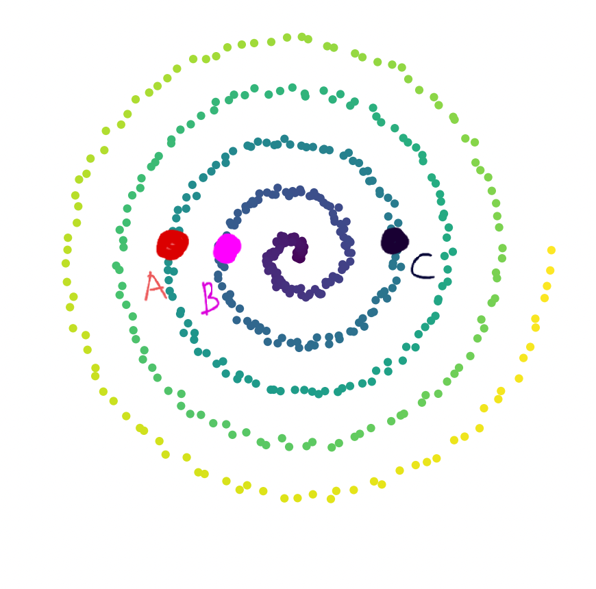
Part 1)
True or False: \(d_{\text{geo}}(A, B) > d_{\text{geo}}(B, C)\).
Solution
True.
Geodesic distance is the distance along the manifold. If we start walking along the 1-dimensional manifold, starting from the center of the spiral, \(B\) comes first, followed by \(C\) and \(A\). Therefore, \(A\) is farther from \(B\) than \(C\) is from \(B\) along the manifold.
Part 2)
True or False: \(d_{\text{geo}}(A, C) > d_{\text{geo}}(A, B)\).
Solution
False.
Along the manifold, the order of the points (starting from the center) is \(B\), \(C\), \(A\). Since \(C\) is between \(B\) and \(A\), the geodesic distance from \(A\) to \(C\) is less than the geodesic distance from \(A\) to \(B\).
Problem #094
Tags: laplacian eigenmaps, quiz-05, optimization, lecture-08
Define the cost function to be:
Consider the similarity matrix with \(n = 3\):
Which of the following embedding vectors \(\vec f\) leads to the minimum cost?
Solution
\((1, 1, 1)^T\).
When \(f_i = f_j\) for all \(i, j\), the term inside the summation is always \(0\), leading the value of the cost function to be \(0\). This is the minimum possible value of the cost function, since all terms in the sum are non-negative.
Problem #095
Tags: laplacian eigenmaps, quiz-05, lecture-08
Given a similarity matrix \(W\) between 3 users:
Create a degree matrix \(D\) from \(W\). What is the value of \(D_{22}\)(the entry in the 2nd row, 2nd column)?
Solution
\(2.4\).
The degree matrix \(D\) is a diagonal matrix where \(D_{ii} = \sum_j W_{ij}\). For \(D_{22}\), we sum the entries of the second row of \(W\):
Problem #096
Tags: laplacian eigenmaps, quiz-05, lecture-08
Consider the similarity matrix:
Find the Graph Laplacian \(L = D - W\). What is the value of \(L_{12}\)(the entry in the 1st row, 2nd column)?
Solution
\(-0.5\).
The Graph Laplacian is \(L = D - W\). Since \(D\) is a diagonal matrix, \(D_{12} = 0\). The similarity \(W_{12} = 0.5\). Therefore:
Problem #097
Tags: lecture-08, laplacian eigenmaps, quiz-05, eigenvalues, eigenvectors
Given a \(4 \times 4\) Graph Laplacian matrix \(L\), the 4 (eigenvalue, eigenvector) pairs of this matrix are given as \((3, \vec v_1)\), \((0, \vec v_2)\), \((8, \vec v_3)\), \((14, \vec v_4)\).
You need to pick one eigenvector. Which of the above eigenvectors will be a non-trivial solution to the spectral embedding problem?
Solution
\(\vec v_1\).
The embedding is the eigenvector with the smallest eigenvalue that is strictly greater than \(0\). The eigenvector \(\vec v_2\) corresponds to eigenvalue \(0\), which gives the trivial solution (all embeddings equal). Among the remaining eigenvectors, \(\vec v_1\) has the smallest eigenvalue (\(3\)), so it is the non-trivial solution to the spectral embedding problem.
Problem #098
Tags: laplacian eigenmaps, quiz-05, lecture-08
Consider a weighted graph of similarity between 3 users. Edges determine the level of similarity between two users (0: least similar, 1: most similar).
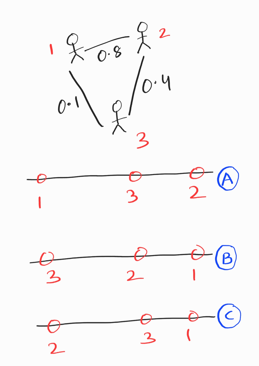
Which option is the best embedding representation for the three users?
Solution
B.
Users 2 and 1 are most similar (highest edge weight), and so they should be closest in the embedding. This makes option B the best choice.
Problem #099
Tags: symmetric matrices, laplacian eigenmaps, quiz-05, lecture-08
True or False: Given a symmetric similarity matrix \(W\), the Graph Laplacian matrix \(L\) will always be symmetric.
Solution
True.
Since \(D\) is a diagonal matrix (and therefore symmetric), and \(W\) is symmetric by assumption, the Graph Laplacian \(L = D - W\) is the difference of two symmetric matrices, which is always symmetric.
Problem #100
Tags: laplacian eigenmaps, quiz-05, lecture-08
Consider the similarity graph shown below.
Part 1)
What is the (1,3) entry of the graph's (unnormalized) Laplacian matrix?
Solution
\(-1/4\).
The Laplacian matrix is \(L = D - W\), where \(W\) is the similarity (adjacency) matrix and \(D\) is the diagonal degree matrix. For off-diagonal entries, \(L_{ij} = -W_{ij}\). Since the weight of the edge between nodes 1 and 3 is \(1/4\), the \((1,3)\) entry of \(L\) is \(-1/4\).
Part 2)
Consider the embedding vector \(\vec f = (1, 2, -1, 4, 8)^T\). What is the cost of this embedding with respect to the Laplacian eigenmaps cost function?
Solution
\(32\).
The cost is \(\displaystyle\text{Cost}(\vec f) = \frac{1}{2}\sum_{i=1}^{n}\sum_{j=1}^{n} w_{ij}(f_i - f_j)^2 = \vec f^T L \vec f\).
If we look at a single edge \((i,j)\) with weight \(w_{ij}\), its contribution to the cost is \(w_{ij}(f_i - f_j)^2\). Thus, we can compute the cost by summing the contributions of all edges in the graph. They are:
The double sum counts each edge twice (once as \((i,j)\) and once as \((j,i)\)), so the \(\frac{1}{2}\) cancels this overcounting, giving \(1 + 1 + 3 + 18 + 5 + 4 = 32\).
Problem #101
Tags: quiz-05, laplacian eigenmaps, eigenvectors, lecture-08
Suppose \(L\) is a graph's Laplacian matrix and let \(\vec f\) be a (nonzero) embedding vector whose embedding cost is zero according to the Laplacian eigenmaps cost function.
True or False: \(\vec f\) is an eigenvector of \(L\).
Solution
True.
If the embedding cost is zero, then \(\vec{f}^T L \vec{f} = 0\). Since \(L\) is positive semidefinite, this implies \(L \vec{f} = \vec{0}\). This means \(\vec{f}\) is an eigenvector of \(L\) with eigenvalue \(0\).
Problem #102
Tags: quiz-05, laplacian eigenmaps, eigenvectors, lecture-08
Suppose a graph \(G\) with nodes \(u_1, \ldots, u_5\) is embedded into \(\mathbb R^2\) using Laplacian Eigenmaps. The bottom three eigenvectors of the graph's Laplacian matrix and their corresponding eigenvalues are:
What is the embedding of node 2?
Solution
\((0, -\frac{2}{\sqrt{6}})^T\).
In Laplacian Eigenmaps, we embed into \(\mathbb{R}^2\) using the eigenvectors corresponding to the two smallest nonzero eigenvalues: \(\vec{u}^{(2)}\)(with \(\lambda_2 = 2\)) and \(\vec{u}^{(3)}\)(with \(\lambda_3 = 5\)). We skip \(\vec{u}^{(1)}\) since it corresponds to \(\lambda_1 = 0\).
The embedding of node \(i\) is \((u^{(2)}_i, u^{(3)}_i)^T\). For node 2 (the second entry of each eigenvector):
Problem #103
Tags: laplacian eigenmaps, quiz-05, lecture-08
Consider the similarity graph shown below.
Part 1)
What is the (1,4) entry of the graph's (unnormalized) Laplacian matrix?
Solution
\(-1/9\).
The Laplacian matrix is \(L = D - W\). For off-diagonal entries, \(L_{ij} = -W_{ij}\). Since the weight of the edge between nodes 1 and 4 is \(1/9\), the \((1,4)\) entry of \(L\) is \(-1/9\).
Part 2)
Consider the embedding vector \(\vec f = (1, 7, 7, -2)^T\). What is the cost of this embedding with respect to the Laplacian eigenmaps cost function?
Solution
\(85\).
The cost is \(\displaystyle\text{Cost}(\vec f) = \frac{1}{2}\sum_{i=1}^{n}\sum_{j=1}^{n} w_{ij}(f_i - f_j)^2 = \vec f^T L \vec f\).
If we look at a single edge \((i,j)\) with weight \(w_{ij}\), its contribution to the cost is \(w_{ij}(f_i - f_j)^2\). Thus, we can compute the cost by summing the contributions of all edges in the graph. They are:
The double sum counts each edge twice (once as \((i,j)\) and once as \((j,i)\)), so the \(\frac{1}{2}\) cancels this overcounting, giving \(18 + 12 + 1 + 0 + 27 + 27 = 85\).
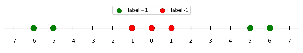
Problem #104
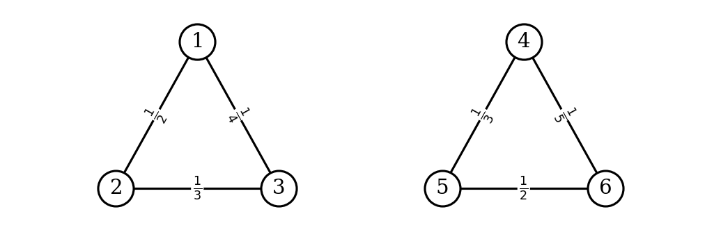
Tags: laplacian eigenmaps, quiz-05, lecture-08
Consider the similarity graph shown below. The weight of each edge is shown; the weight of non-existing edges is zero.
Is \(\vec f = (3, 3, 3, -2, -2, -2)^T\) an eigenvector of the graph's Laplacian matrix? If so, what is its eigenvalue?
Solution
Yes, \(\vec f\) is an eigenvector of the Laplacian with eigenvalue \(\lambda = 0\).
To verify, we could\(L \vec f\) and check that it is \(\vec 0\), but there's an easier way to see this.
The vector \(\vec f\) assigns the same value to nodes \(\{1, 2, 3\}\) and another same value to nodes \(\{4, 5, 6\}\). This means that it is embedding all of the nodes in the first connected component to the same point, and all of the nodes in the second connected component to another same point.
When we think of the cost of this embedding with respect to the Laplacian Eigenmaps cost function, we see that the cost is zero. This is because any term where \(W_{ij} > 0\) comes from two nodes in the same connected component, and for them \(f_i = f_j\), so \((f_i - f_j)^2 = 0\). For any pair of nodes, one in the first component and one in the second, \(W_{ij} = 0\), so they do not contribute to the cost, no matter what their \(f\) values are.
Since the cost is zero, we have \(\vec f^T L \vec f = 0\). This implies that \(L \vec f = \vec 0\), so \(\vec f\) is an eigenvector of \(L\) with eigenvalue \(\lambda = 0\).
This will happen any time we have an unweighted graph with multiple connected components: there will be multiple eigenvectors with eigenvalue \(0\), each corresponding to an embedding that assigns a different constant value to each connected component.
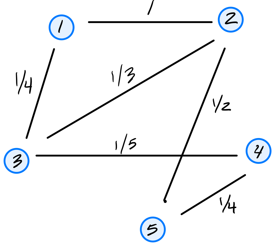
Problem #105
Tags: laplacian eigenmaps, quiz-05, lecture-08
Consider the similarity graph shown below.

Part 1)
What is the (2,2) entry of the graph's (unnormalized) Laplacian matrix?
Solution
\(11/6\).
The Laplacian matrix is \(L = D - W\), where \(W\) is the similarity (adjacency) matrix and \(D\) is the diagonal degree matrix. For diagonal entries, \(L_{ii} = d_i\), the degree of node \(i\). Node 2 is connected to nodes 1, 3, and 5 with weights \(1\), \(1/3\), and \(1/2\), respectively, so \(d_2 = 1 + 1/3 + 1/2 = 11/6\).
Part 2)
Consider the embedding vector \(\vec f = (3, 0, -3, 2, 6)^T\). What is the cost of this embedding with respect to the Laplacian eigenmaps cost function?
Solution
\(48\).
The cost is \(\displaystyle\text{Cost}(\vec f) = \frac{1}{2}\sum_{i=1}^{n}\sum_{j=1}^{n} w_{ij}(f_i - f_j)^2 = \vec f^T L \vec f\).
If we look at a single edge \((i,j)\) with weight \(w_{ij}\), its contribution to the cost is \(w_{ij}(f_i - f_j)^2\). Thus, we can compute the cost by summing the contributions of all edges in the graph. They are:
The double sum counts each edge twice (once as \((i,j)\) and once as \((j,i)\)), so the \(\frac{1}{2}\) cancels this overcounting, giving \(9 + 9 + 3 + 18 + 5 + 4 = 48\).
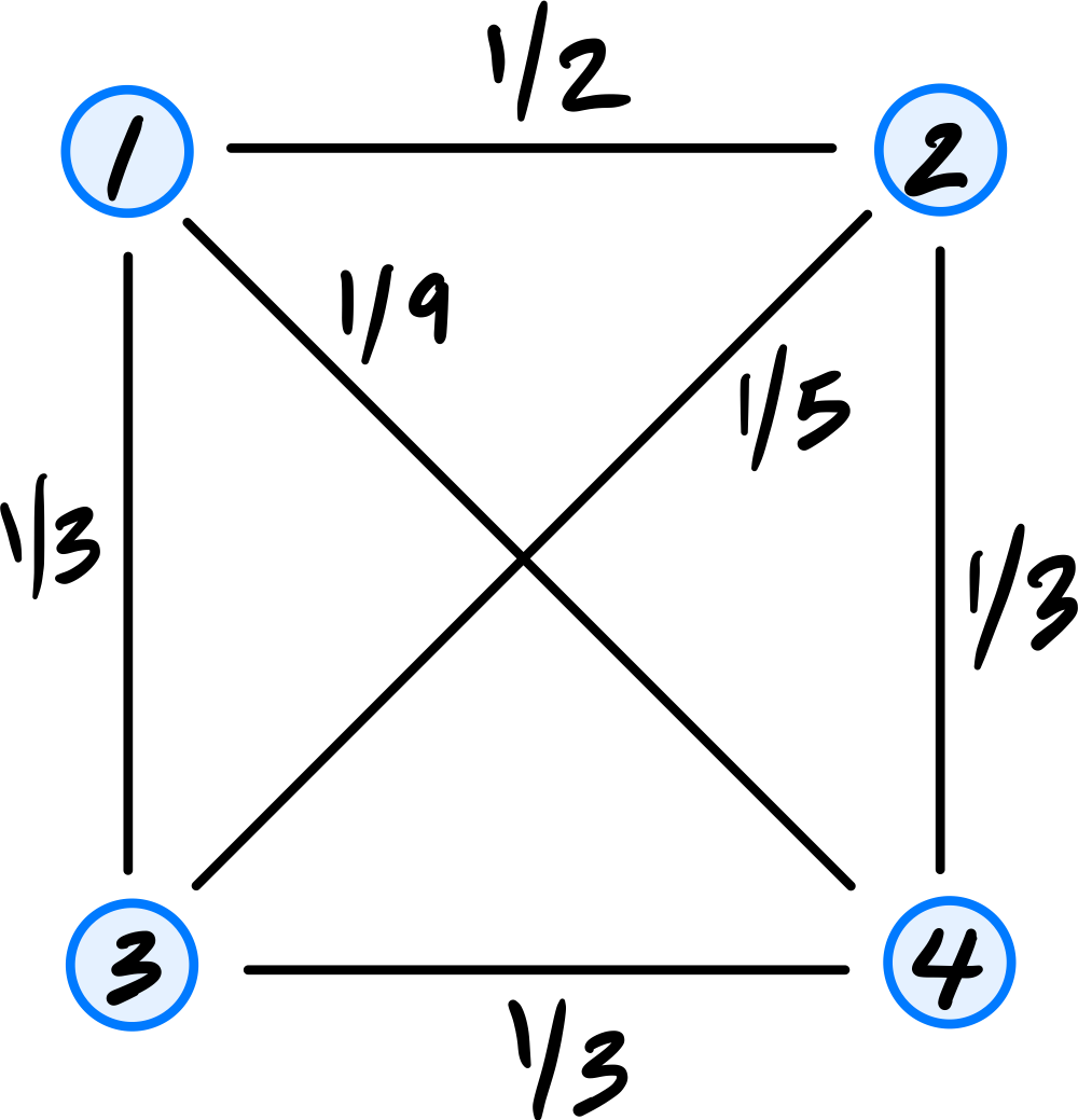
Problem #106
Tags: laplacian eigenmaps, quiz-05, lecture-08
Consider the similarity graph shown below.

Part 1)
What is the (3,4) entry of the graph's (unnormalized) Laplacian matrix?
Solution
\(-1/5\).
The Laplacian matrix is \(L = D - W\), where \(W\) is the similarity (adjacency) matrix and \(D\) is the diagonal degree matrix. For off-diagonal entries, \(L_{ij} = -W_{ij}\). Since the weight of the edge between nodes 3 and 4 is \(1/5\), the \((3,4)\) entry of \(L\) is \(-1/5\).
Part 2)
Consider the embedding vector \(\vec f = (2, 3, 0, 5, -1)^T\). What is the cost of this embedding with respect to the Laplacian eigenmaps cost function?
Solution
\(27\).
The cost is \(\displaystyle\text{Cost}(\vec f) = \frac{1}{2}\sum_{i=1}^{n}\sum_{j=1}^{n} w_{ij}(f_i - f_j)^2 = \vec f^T L \vec f\).
If we look at a single edge \((i,j)\) with weight \(w_{ij}\), its contribution to the cost is \(w_{ij}(f_i - f_j)^2\). Thus, we can compute the cost by summing the contributions of all edges in the graph. They are:
The double sum counts each edge twice (once as \((i,j)\) and once as \((j,i)\)), so the \(\frac{1}{2}\) cancels this overcounting, giving \(1 + 1 + 3 + 8 + 5 + 9 = 27\).
Problem #107
Tags: quiz-05, laplacian eigenmaps, eigenvectors, lecture-08
Suppose a graph \(G\) with nodes \(u_1, \ldots, u_5\) is embedded into \(\mathbb R^2\) using Laplacian Eigenmaps. The bottom three eigenvectors of the graph's Laplacian matrix and their corresponding eigenvalues are:
What is the embedding of node 4?
Solution
\((-\frac{1}{\sqrt{2}}, \frac{1}{\sqrt{6}})^T\).
In Laplacian Eigenmaps, we embed into \(\mathbb{R}^2\) using the eigenvectors corresponding to the two smallest nonzero eigenvalues: \(\vec{u}^{(2)}\)(with \(\lambda_2 = 3\)) and \(\vec{u}^{(3)}\)(with \(\lambda_3 = 7\)). We skip \(\vec{u}^{(1)}\) since it corresponds to \(\lambda_1 = 0\).
The embedding of node \(i\) is \((u^{(2)}_i, u^{(3)}_i)^T\). For node 4 (the fourth entry of each eigenvector):
Problem #108
Tags: quiz-05, lecture-09, feature maps
Suppose you are given the following basis functions that define a feature map \(\vec\phi: \mathbb{R}^3 \to\mathbb{R}^4\):
What is the representation of the data point \(\vec{x} = (3, 2, -1)\) in the new feature space?
Solution
\((6, 4, 3, -6)\).
We compute each basis function at \(\vec{x} = (3, 2, -1)\):
So \(\vec\phi(\vec{x}) = (6, 4, 3, -6)\).
Problem #109
Tags: quiz-05, lecture-09, feature maps
Suppose you are given the following basis functions that define a feature map \(\vec\phi: \mathbb{R}^3 \to\mathbb{R}^4\):
What is the representation of the data point \(\vec{x} = (2, -1, 3)\) in the new feature space?
Solution
\((4, -3, 6, 3)\).
We compute each basis function at \(\vec{x} = (2, -1, 3)\):
So \(\vec\phi(\vec{x}) = (4, -3, 6, 3)\).
Problem #110
Tags: quiz-05, lecture-09, feature maps
Suppose you are given the following basis functions that define a feature map \(\vec\phi: \mathbb{R}^3 \to\mathbb{R}^4\):
What is the representation of the data point \(\vec{x} = (2, -3, 1)\) in the new feature space?
Solution
\((9, 2, -3, 4)\).
We compute each basis function at \(\vec{x} = (2, -3, 1)\):
So \(\vec\phi(\vec{x}) = (9, 2, -3, 4)\).
Problem #111
Tags: linear classifiers, quiz-05, lecture-09, feature maps
Suppose we have a feature map \(\varphi : \mathbb{R}^3 \to\mathbb{R}^4\) with the following basis functions:
A linear classifier in this feature space has learned the weight vector \(\vec{w} = (w_0, w_1, w_2, w_3, w_4) = (0.4,\; 0.3,\; -0.6,\; 1.3,\; 0.7)\), where \(w_0 = 0.4\) is the bias (intercept) term. The prediction function is:
What is the value of the prediction function \(H\) for the input point \(\vec{x} = (3, 2, -1)\) in the original \(\mathbb{R}^3\) space?
Solution
\(-0.5\).
First, we compute the feature representation of \(\vec{x} = (3, 2, -1)\):
So the feature vector is \(\varphi(\vec{x}) = (6, 4, 3, -6)\).
Then we compute the prediction function:
Problem #112
Tags: linear classifiers, quiz-05, lecture-09, feature maps
Suppose we have a feature map \(\varphi : \mathbb{R}^3 \to\mathbb{R}^4\) with the following basis functions:
A linear classifier in this feature space has learned the weight vector \(\vec{w} = (w_0, w_1, w_2, w_3, w_4) = (0.5,\; 0.25,\; -1,\; 0.5,\; -0.5)\), where \(w_0 = 0.5\) is the bias (intercept) term. The prediction function is:
What is the value of the prediction function \(H\) for the input point \(\vec{x} = (2, -1, 3)\) in the original \(\mathbb{R}^3\) space?
Solution
\(6\).
First, we compute the feature representation of \(\vec{x} = (2, -1, 3)\):
So the feature vector is \(\varphi(\vec{x}) = (4, -3, 6, 3)\).
Then we compute the prediction function:
Problem #113
Tags: linear classifiers, quiz-05, lecture-09, feature maps
Suppose we have a feature map \(\varphi : \mathbb{R}^3 \to\mathbb{R}^4\) with the following basis functions:
A linear classifier in this feature space has learned the weight vector \(\vec{w} = (w_0, w_1, w_2, w_3, w_4) = (2,\; -1,\; 3,\; 0.5,\; -2)\), where \(w_0 = 2\) is the bias (intercept) term. The prediction function is:
What is the value of the prediction function \(H\) for the input point \(\vec{x} = (1, -3, 2)\) in the original \(\mathbb{R}^3\) space?
Solution
\(-4.5\).
First, we compute the feature representation of \(\vec{x} = (1, -3, 2)\):
So the feature vector is \(\varphi(\vec{x}) = (4, 2, 3, 5)\).
Then we compute the prediction function:
Problem #114
Tags: linear classifiers, quiz-05, lecture-09, feature maps
Consider the following data in \(\mathbb{R}\):
Note that this data is not linearly separable in \(\mathbb{R}\). For each of the following transformations that map the data into \(\mathbb{R}^2\), determine whether the transformed data is linearly separable.
Part 1)
True or False: The transformation \(x \mapsto(x, x^3)\) makes the data linearly separable in \(\mathbb{R}^2\).
Solution
False.
Since \(x^3\) is a monotonically increasing function, the relative order of the points along the curve \(y = x^3\) is the same as in 1D. The classes remain interleaved and cannot be separated by a line.
Part 2)
True or False: The transformation \(x \mapsto(x, x^2)\) makes the data linearly separable in \(\mathbb{R}^2\).
Solution
True.
The green points have large \(x^2\) values (\(25\) and \(36\)) while the red points have small \(x^2\) values (\(0\) and \(1\)). A horizontal line such as \(x_2 = 10\) separates them.
Part 3)
True or False: The transformation \(x \mapsto(x, |x|)\) makes the data linearly separable in \(\mathbb{R}^2\).
Solution
True.
The green points have large \(|x|\) values (\(5\) and \(6\)) while the red points have small \(|x|\) values (\(0\) and \(1\)). A horizontal line such as \(x_2 = 3\) separates them.
Part 4)
True or False: The transformation \(x \mapsto(x, x)\) makes the data linearly separable in \(\mathbb{R}^2\).
Solution
False.
This transformation maps every point to the line \(y = x\) in \(\mathbb{R}^2\). The data is effectively still one-dimensional, and the classes remain interleaved along this line.
Problem #115
Tags: linear classifiers, quiz-05, lecture-09, feature maps
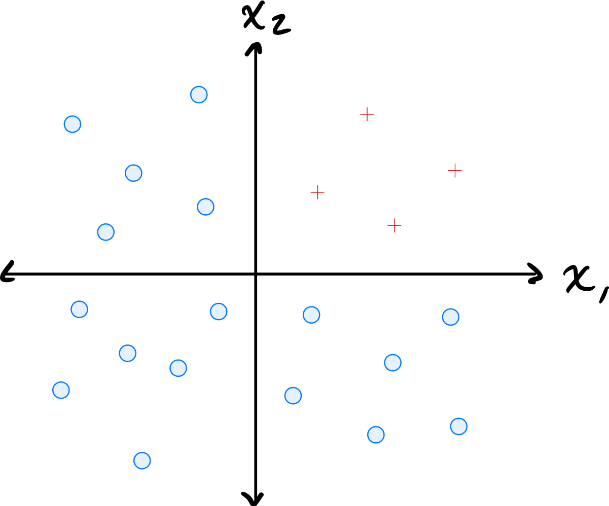
Consider the data shown below:
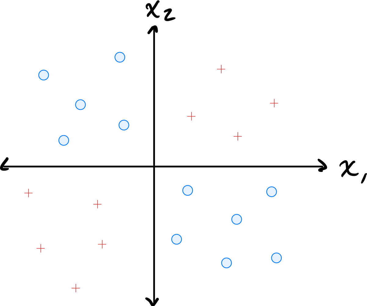
The data comes from two classes: \(\circ\) and \(+\).
Suppose a single basis function will be used to map the data to feature space where a linear classifier will be trained. Which of the below is the best choice of basis function?
Solution
\(\varphi(x_1, x_2) = x_1 \cdot x_2\).
The data has \(\circ\) points in quadrants where \(x_1\) and \(x_2\) have the same sign (so \(x_1 x_2 > 0\)) and \(+\) points where they have opposite signs (so \(x_1 x_2 < 0\)). The product \(x_1 \cdot x_2\) captures this separation, allowing a linear classifier in the 1D feature space to distinguish the classes.
Problem #116
Tags: linear classifiers, quiz-05, lecture-09, feature maps
Define the "triangle" basis function:
Three triangle basis functions \(\phi_1\), \(\phi_2\), \(\phi_3\) have centers \(c_1 = 1\), \(c_2 = 4\), and \(c_3 = 5\), respectively. These basis functions map data from \(\mathbb{R}\) to feature space \(\mathbb{R}^3\) via \(x \mapsto(\phi_1(x), \phi_2(x), \phi_3(x))^T\).
A linear predictor in feature space has equation:
Part 1)
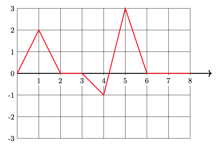
What is the representation of \(x = 4.5\) in feature space?
Solution
\((0, 1/2, 1/2)^T\).
We evaluate each basis function at \(x = 4.5\):
Therefore, the feature space representation is \((0, 1/2, 1/2)^T\).
Part 2)
What is \(H(4.5)\) in the original space?
Solution
\(1\).
Using the feature space representation from part (a):
Part 3)
Plot \(H(x)\)(the prediction function in the original space) from 0 to 8 on the grid below.
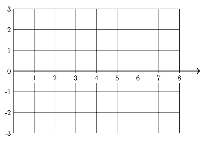
Solution
Problem #117
Tags: linear classifiers, quiz-05, lecture-09, feature maps
Consider the data shown below:
The data comes from two classes: \(\circ\) and \(+\).
Suppose a single basis function will be used to map the data to feature space where a linear classifier will be trained. Which of the below is the best choice of basis function?
Solution
\(\varphi(x_1, x_2) = \min\{x_1, x_2\}\).
The data has \(\circ\) points where both coordinates are large and \(+\) points where at least one coordinate is small. The minimum of the two coordinates captures this: \(\circ\) points have a large minimum while \(+\) points have a small minimum. This allows a linear classifier in the 1D feature space to separate the classes.
Problem #118
Tags: linear classifiers, quiz-05, lecture-09, feature maps
Define the "box" basis function:
Three box basis functions \(\phi_1\), \(\phi_2\), \(\phi_3\) have centers \(c_1 = 1\), \(c_2 = 2\), and \(c_3 = 6\), respectively. These basis functions map data from \(\mathbb{R}\) to feature space \(\mathbb{R}^3\) via \(x \mapsto(\phi_1(x), \phi_2(x), \phi_3(x))^T\).
A linear predictor in feature space has equation:
Part 1)
What is the representation of \(x = 1.5\) in feature space?
Solution
\((1, 1, 0)^T\).
We evaluate each basis function at \(x = 1.5\):
Therefore, the feature space representation is \((1, 1, 0)^T\).
Part 2)
What is \(H(2.5)\)?
Solution
\(-1\).
First, we find the feature space representation of \(x = 2.5\):
Then:
Part 3)
Plot \(H(x)\)(the prediction function in the original space) from 0 to 8 on the grid below.

Solution
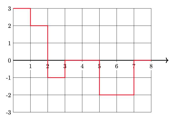
Problem #119
Tags: quiz-05, RBF networks, lecture-10
Suppose a Gaussian RBF network \(H(\vec x) : \mathbb{R}^2 \to\mathbb{R}\) is trained on a binary classification dataset using four Gaussian RBFs located at \(\vec\mu_1 = (0,0)\), \(\vec\mu_2 = (1,0)\), \(\vec\mu_3 = (0,1)\), and \(\vec\mu_4 = (1,1)\).
All four RBFs use the same width parameter, \(\sigma\).
After training, it is found that the weights corresponding to the four basis functions are \(w_1 = -3\), \(w_2 = 3\), \(w_3 = 3\), \(w_4 = -3\).
Which of the below could show the decision boundary of \(H\)? The plusses and minuses show where the prediction function, \(H\), is positive and negative.
Solution
The second plot is correct.
The weights \(w_2 = 3\) and \(w_3 = 3\) are positive at \((1,0)\) and \((0,1)\), while \(w_1 = -3\) and \(w_4 = -3\) are negative at \((0,0)\) and \((1,1)\). This means \(H\) is positive near \((1,0)\) and \((0,1)\) and negative near \((0,0)\) and \((1,1)\). The decision boundary separates these regions, running diagonally through the square.
Problem #120
Tags: lecture-10, quiz-05, RBF networks, feature maps
Let \(\mathcal{X} = \{(\vec{x}^{(1)}, y_1), \ldots, (\vec{x}^{(100)}, y_{100})\}\) be a dataset of 100 points, where each feature vector \(\vec{x}^{(i)}\in\mathbb{R}^{50}\). Suppose a Gaussian RBF network is trained using 25 Gaussian basis functions.
Recall that a Gaussian RBF network can be viewed as mapping the data to feature space, where a linear prediction rule is trained. In the above scenario, what is the dimensionality of this feature space?
Solution
\(25\).
Each Gaussian basis function produces one feature (the output of that basis function applied to the input). With 25 basis functions, the feature space is \(\mathbb{R}^{25}\). The dimensionality of the feature space equals the number of basis functions, not the original input dimension.
Problem #121
Tags: quiz-05, RBF networks, lecture-10
Does standardizing features affect the output of a Gaussian RBF network?
More precisely, let \(\mathcal{X} = \{(\vec{x}^{(1)}, y_1), \ldots, (\vec{x}^{(n)}, y_n)\}\) be a dataset, and let \(\mathcal{Z} = \{(\vec{z}^{(1)}, y_1), \ldots, (\vec{z}^{(n)}, y_n)\}\) be the dataset obtained by standardizing each feature in \(\mathcal{X}\)(that is, each feature is scaled to have unit standard deviation and zero mean). Note that the \(y_i\)'s are not standardized -- they are the same in both datasets.
Suppose \(H_\mathcal{X}(\vec{x})\) is a Gaussian RBF network trained by minimizing mean squared error on \(\mathcal{X}\), and \(H_\mathcal{Z}(\vec{z})\) is a Gaussian RBF network trained by minimizing mean squared error on \(\mathcal{Z}\). Both RBF networks use the same width parameters, \(\sigma\). The centers used in \(H_\mathcal{Z}\) are obtained by standardizing the centers used in \(H_\mathcal{X}\) using the mean and standard deviation of the data, \(\vec{x}^{(i)}\).
True or False: it must be the case that \(H_\mathcal{X}(\vec{x}^{(i)}) = H_\mathcal{Z}(\vec{z}^{(i)})\) for all \(i \in\{1, \ldots, n\}\).
Solution
False.
Standardizing changes the distances between points and centers. The Gaussian basis function \(\varphi(\vec{x}; \vec{\mu}, \sigma) = e^{-\|\vec{x} - \vec{\mu}\|^2 / \sigma^2}\) depends on the Euclidean distance \(\|\vec{x} - \vec{\mu}\|\). While the centers are standardized along with the data, the width parameter \(\sigma\) remains the same. Since standardizing changes the scale of the features (and thus the distances), using the same \(\sigma\) will produce different basis function outputs, leading to different predictions.
Problem #122
Tags: quiz-05, RBF networks, lecture-10
Consider the following labeled data set of three points:
A Gaussian RBF network \(H(x) : \mathbb{R}\to\mathbb{R}\) is trained on this data with two Gaussian basis functions of the form \(\varphi_i(x; \mu_i, \sigma_i) = e^{-(x - \mu_i)^2 / \sigma_i^2}\). The centers of the basis functions are at \(\mu_1 = 2\) and \(\mu_2 = 6\), and both use a width parameter of \(\sigma = \sigma_1 = \sigma_2 = 1\).
Suppose the RBF network does not have a bias parameter, so that the prediction function is \(H(x) = w_1 \varphi_1(x) + w_2 \varphi_2(x)\).
What is \(w_1\), approximately? Your answer may involve \(e\), but should evaluate to a number.
Solution
\(w_1 \approx 3e\).
We evaluate the basis functions at each data point. Note that when a basis function center is far from a data point, the Gaussian evaluates to approximately zero.
At \(x_1 = 1\): \(\varphi_1(1) = e^{-(1-2)^2} = e^{-1}\) and \(\varphi_2(1) = e^{-(1-6)^2} = e^{-25}\approx 0\).
At \(x_3 = 6\): \(\varphi_1(6) = e^{-(6-2)^2} = e^{-16}\approx 0\) and \(\varphi_2(6) = e^{0} = 1\).
So \(H(1) \approx w_1 e^{-1} = y_1 = 3\), giving \(w_1 \approx 3e\). Similarly, \(H(6) \approx w_2 = y_3 = 3\), confirming \(w_2 \approx 3\).
Problem #123
Tags: lecture-10, quiz-05, RBF networks, feature maps
Consider a Gaussian RBF network with three basis functions of the form \(\varphi_i(\vec x) = e^{-\|\vec x - \vec \mu^{(i)}\|^2 / \sigma^2}\), where \(\sigma = 2\) for all basis functions. The centers \(\vec\mu^{(1)}\), \(\vec\mu^{(2)}\), and \(\vec\mu^{(3)}\) are shown as black \(\times\) markers in the figure below.
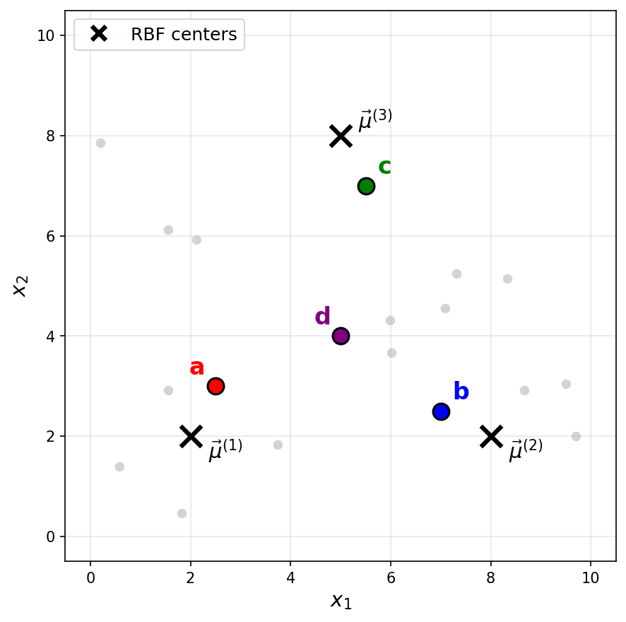
Recall that a Gaussian RBF network can be viewed as mapping data points to a feature space, where the new representation of a point \(\vec x\) is:
Suppose a point \(\vec x\) has the following feature representation:
Which of the labeled points (a, b, c, or d) could be \(\vec x\)?
Solution
The answer is c.
The feature representation tells us that \(\varphi_1(\vec x) \approx 0\), \(\varphi_2(\vec x) \approx 0\), and \(\varphi_3(\vec x) \approx 0.73\).
Since a Gaussian basis function \(\varphi_i(\vec x) = e^{-\|\vec x - \vec \mu^{(i)}\|^2 / \sigma^2}\) outputs values close to 1 when \(\vec x\) is near the center \(\vec\mu^{(i)}\) and values close to 0 when \(\vec x\) is far from the center, the feature representation indicates that \(\vec x\) is far from \(\vec\mu^{(1)}\) and \(\vec\mu^{(2)}\)(since \(\varphi_1 \approx 0\) and \(\varphi_2 \approx 0\)), but relatively close to \(\vec\mu^{(3)}\)(since \(\varphi_3 \approx 0.73\)).
Looking at the figure, point c is the only point that is close to \(\vec\mu^{(3)}\) and far from both \(\vec\mu^{(1)}\) and \(\vec\mu^{(2)}\).
Problem #124
Tags: lecture-10, quiz-05, RBF networks, feature maps
Consider a Gaussian RBF network with three basis functions of the form \(\varphi_i(\vec x) = e^{-\|\vec x - \vec \mu^{(i)}\|^2 / \sigma^2}\), where \(\sigma = 3\) for all basis functions. The centers \(\vec\mu^{(1)}\), \(\vec\mu^{(2)}\), and \(\vec\mu^{(3)}\) are shown as black \(\times\) markers in the figure below.
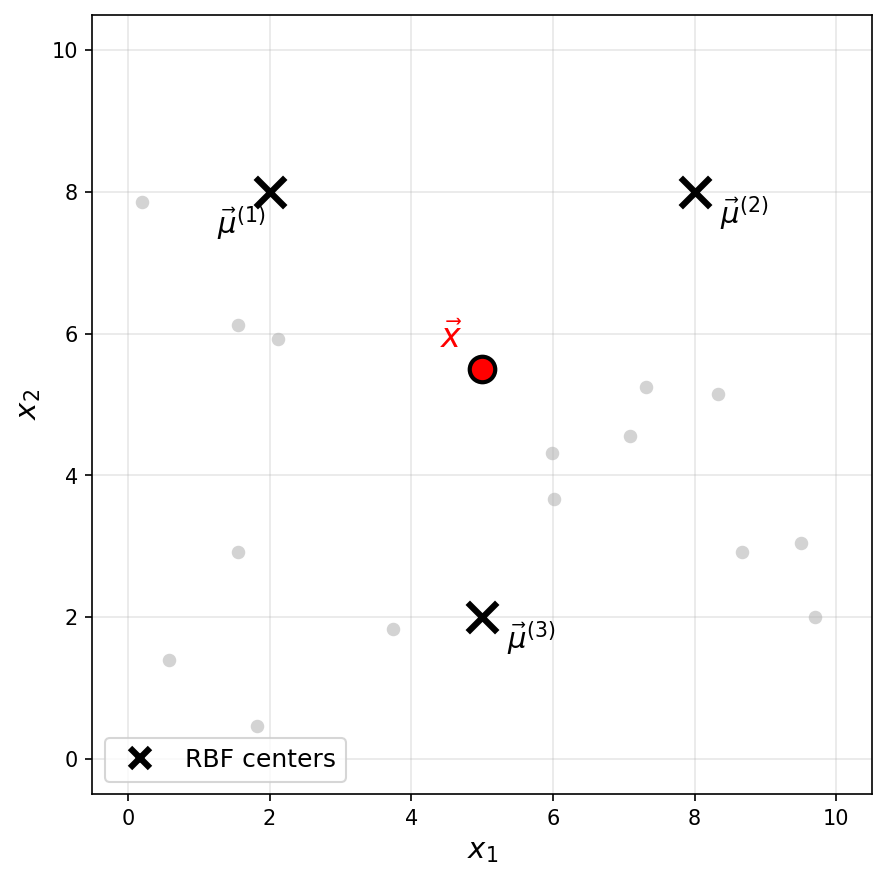
Recall that a Gaussian RBF network can be viewed as mapping data points to a feature space, where the new representation of a point \(\vec x\) is:
One of the following is the feature representation of the highlighted point \(\vec x\). Which one?
Solution
The answer is \(\vec f(\vec x) \approx(0.18, 0.18, 0.26)^T\).
The highlighted point \(\vec x\) is not particularly close to any of the three centers. It is roughly equidistant from \(\vec\mu^{(1)}\) and \(\vec\mu^{(2)}\), and slightly closer to \(\vec\mu^{(3)}\).
Since a Gaussian basis function outputs values close to 1 only when the input is very near the center and decays toward 0 as the distance increases, we expect all three basis functions to output moderate, nonzero values. This rules out the first three options, which each have one large value and two zeros (corresponding to a point very close to a single center).